VMD and CPPTRAJ Basics for Visualization and Analysis of MD Trajectories

Lauren Lerew¹ and Darrin M. York^1
1Laboratory for Biomolecular Simulation Research, Institute for Quantitative Biomedicine and Department of Chemistry and Chemical Biology, Rutgers University, Piscataway, NJ 08854, USA

Learning objectives

Outline

• 1.1 VMD Overview
• 1.2 How to Access VMD
• 1.3 VMD Basics
• 1.4 Customizing Representations
• 1.5 Measuring Geometrical Properties
• 1.6 Keywords and Aligning
• 1.7 Calculating Root-Mean-Square Deviation (RMSD)
• 1.8 Image Rendering
• 2.1 Introduction to CPPTRAJ
• 2.2 Wrapping Trajectories
• 2.3 Trajectory Time Series and Distribution Analysis
• 2.4 Computing Average Structures and Fluctuations

1.1 VMD Overview

VMD is a powerful high-performance, cross-platform molecular graphics viewer developed by the Theoretical and Computational Biophysics Group (TCBG) that is widely used (among other things) for displaying static and dynamic structures, viewing sequence information, and performing dynamic analysis. There is an online User's Guide as well as a number of detailed tutorials available. Further support is provided by the VMD Mailing List.

1.2 How to Access VMD

VMD is accessible through Expanse, or can be downloaded and run locally on your laptop or workstation.

To access from Expanse:

[user@expanse] module spider vmd

[user@expanse] vmd

To Download and Install on your Local Computer:

If you are having trouble using VMD on a Windows machine, you can install ubuntu as a Windows subsystem for linux (wsl) and install VMD there. A quick guide to do so can be found here.

1.3 VMD Basics

This tutorial will introduce you to the 3 systems that will be used throughout the remainder of the tutorials:

The goal for this tutorial is to practice using both VMD and CPPTRAJ to obtain a visual understanding of each system.

All of the input files for this tutorial can be found in /expanse/projects/qstore/amber_ws/tutorials/VMD_CPPTRAJ_Basics/input_files. Please copy them to your working directory. Additionally, all output files produced by this tutorial can be found in /expanse/projects/qstore/amber_ws/tutorials/VMD_CPPTRAJ_Basics/output_files should you need to access them. You will begin by loading one of our simplest systems, an acetic acid molecule in a solution of water and ions. To do so:

Loading Through Expanse:

[user@expanse] vmd centered.acetic_acid_aq.pdb

Loading Through Personal Computer GUI:

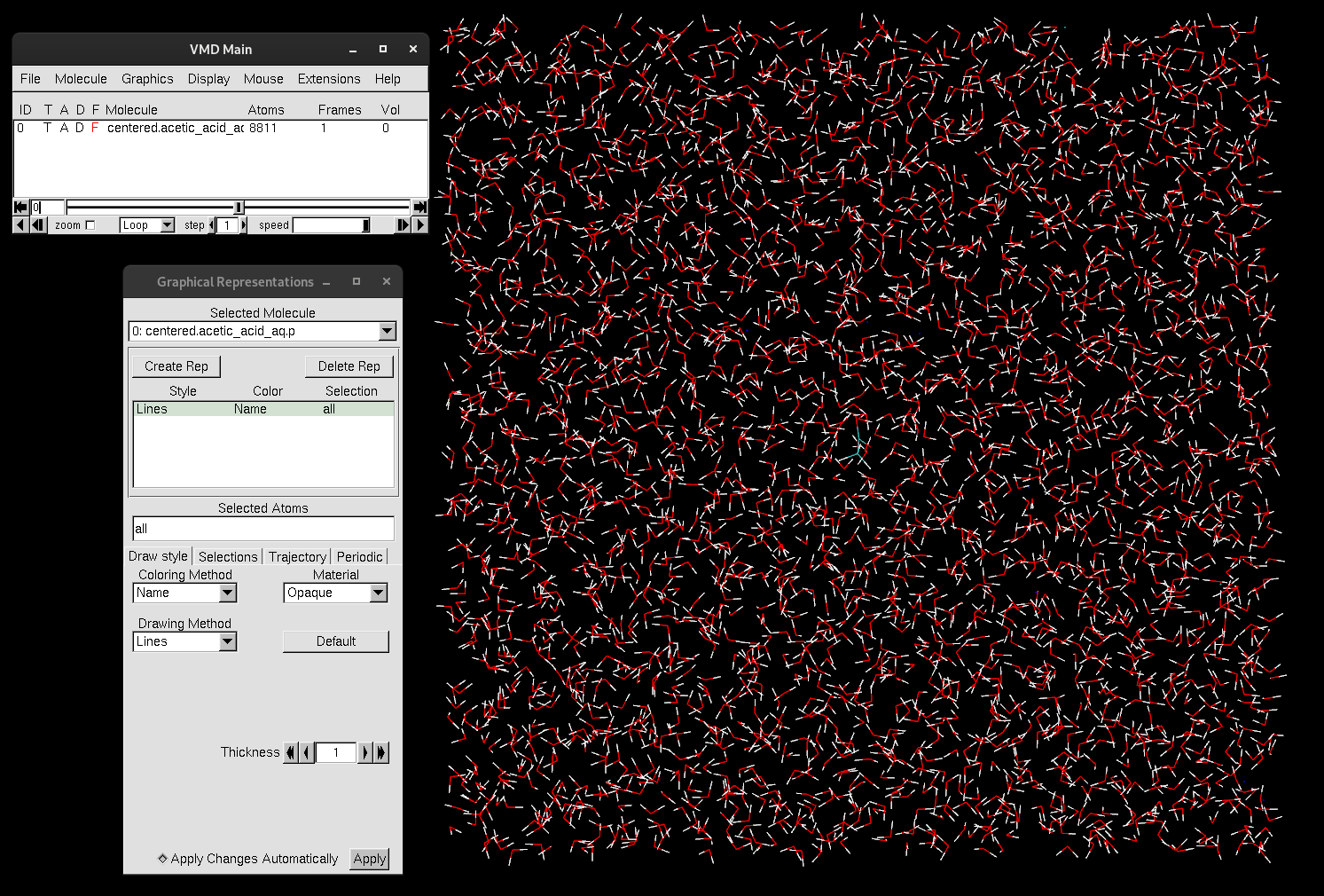
You should see something like this:

As you can see, VMD consists of 3 windows:

1. Display
2. VMD Main
3. Graphical Representations

The VMD Main is the control window for VMD, and you see which molecules are loaded.

VMD contains a lot of gadgets and options for visualization and analysis, so carefully float your mouse over each menu option in the VMD Main to briefly explore the sub-menus. For example,if you go into the Display menu, you can change the settings of the display...play around with different settings to see how it affects how the system is displayed.

Moving the molecule around in VMD is quite easy; you have the option of going through the Mouse menu, or through keyboard shortcuts:

To rotate molecule:r
 
To translate molecule: t
To scale (zoom-in or out): s
To center the system in the display: =

1.4 Customizing Representations

Representations are used to separate out the individual components within the system, such as distinguishing the acetic acid (solute) from the surrounding waters and ions (solvent).

The Graphical Representations window is typically already up on your screen, but if it is not, selecting it will cause it to appear. This window provides a wide range of different ways to visually represent the molecules in your system, allowing for a more meaningful analysis of the structural organization and interactions.

At the top, you can see which system is selected. If you have multiple systems loaded, you can use the down arrow to toggle through them and view the representations for each system. For now, we only have one system loaded. There are two buttons under Create Rep and Delete Rep. The Create Rep will create a new representation, while the Delete Rep will delete. If you want to simply turn off a representation, double-click on the representation. It will turn red and be off. The Selected Atoms box is where you type what will be your selection for the representation at hand. Underneath that are four tabs:

1. Draw style
2. Selections
3. Trajectory
4. Periodic

Draw style is where you have the creative ability to change how the selection is represented. The Coloring Method is where you define how the colors are assigned to molecules. The Drawing Method determines the shapes of its atoms, bonds and other components. And the Material can change shading or how the objects appear. The default representation selection is all. If you need additional guidance on the available selection types, the Selections tab provides a list of options that you can browse. When a trajectory is loaded into VMD, you can smooth the animation by changing the settings under the Trajectory tab. Lastly, the Periodic tab is a good place to check if your periodic unit cell box is properly established. Here you can display multiple unit cells.

You should see now that only ions and the acetic acid are selected and displayed:

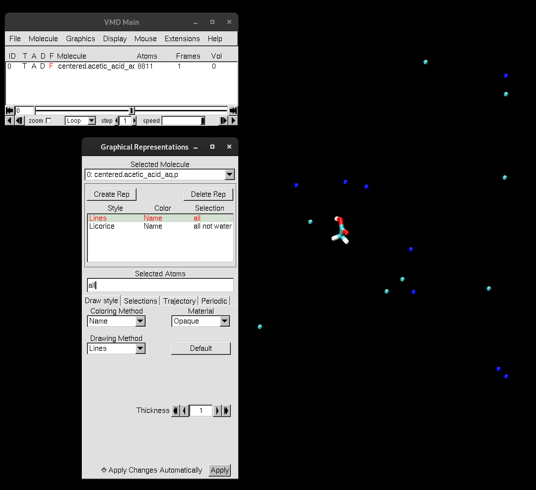
Now, create a representation to select only the acetic acid.

1.5 Measuring Geometrical Properties

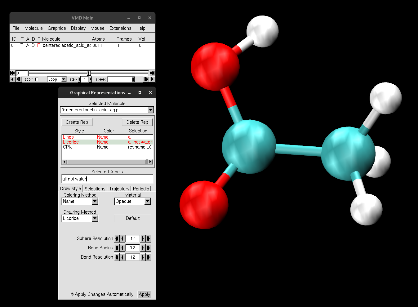
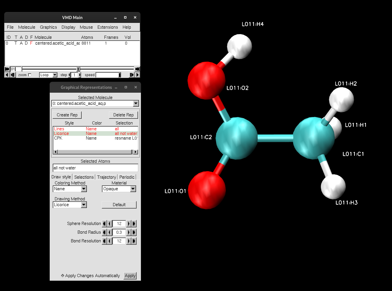
Here, you can switch-on selection modes to label atoms, bonds or angles in order to obtain metrics about the system. You can either use the selections seen in the sub-menu or you can use these keyboard shortcuts:

To select an atom, press 1 and then make your selection. It will add a label that contains the residue ID and the atom name.
To select and measure a bond distance between two atoms, press 2. First click on one atom, then click on the other. The distance between the two atoms will pop up in Å.
To select and measure an angle, press 3 and carefully select three atoms of choice. A label for the angle will be displayed.
To select and measure a dihedral angle between four atoms, press 4 and carefully select the atoms. A label for the angle will be displayed.

You should get very comfortable switching between the different selection types using the keyboard.

With the labels displayed, you can now see that the acetic acid molecule is identified by the name "L01":

A helpful keyword for selecting and finding atoms within a certain distance is "within".

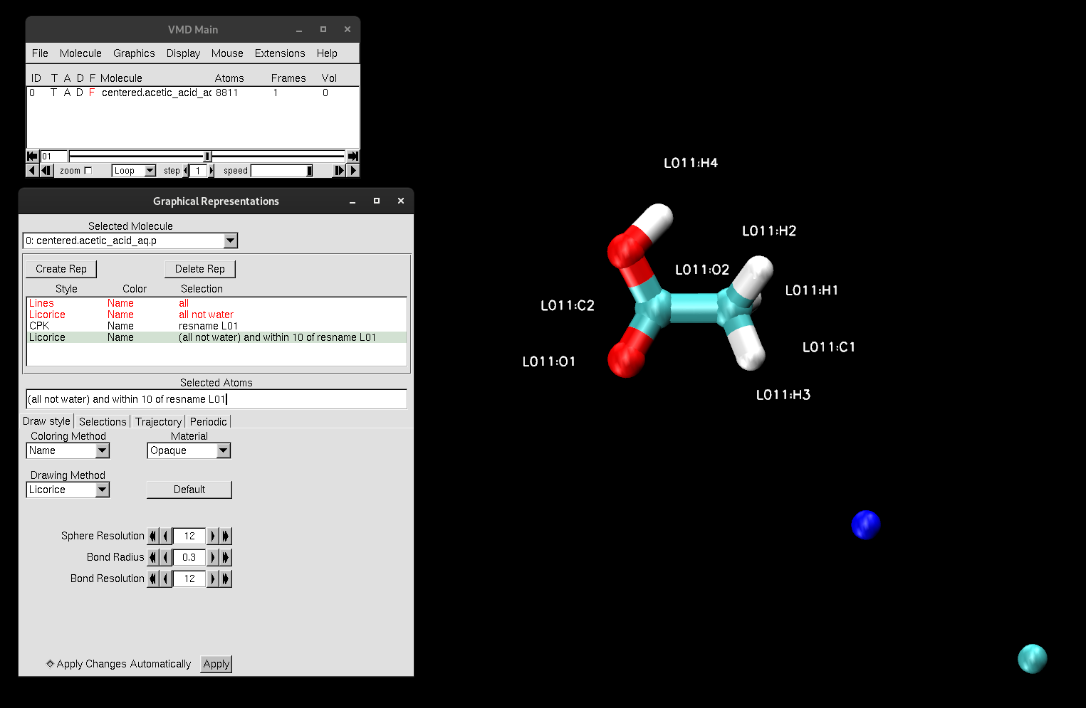
This selection will select only the ions that are within 10 Å, due to the selection in parentheses "all not water".

From here, use the bond selection tool (2 on the keyboard) to label the distance of the closest ion.

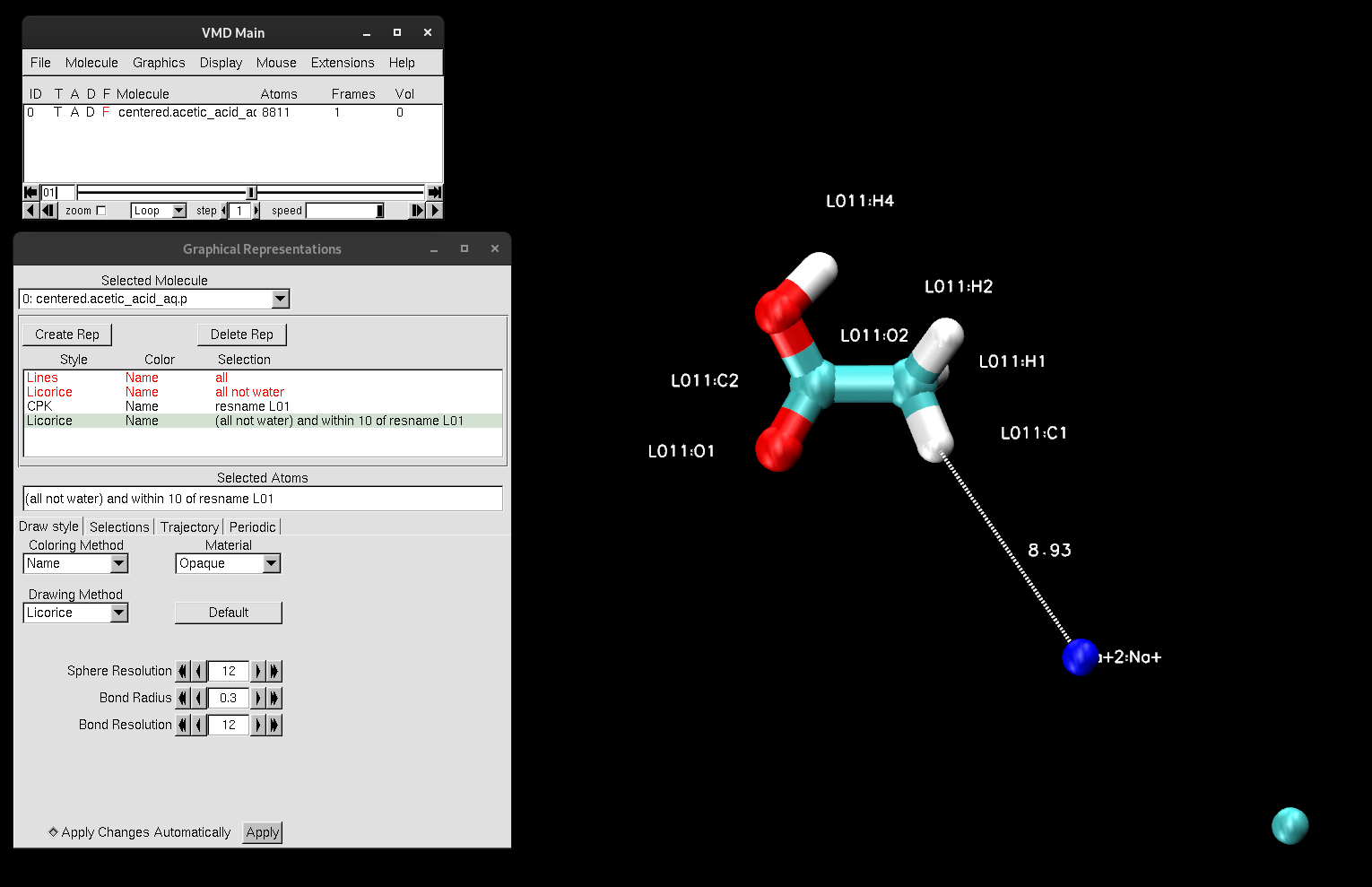
Try measuring the dihedral angle between H4, O2, C2, and C1

All of the labels that you create are stored under Graphics → Labels. Here, you can find more specifications regarding the atom, bond or angle that you had labeled. For example, you can see what residue a labeled atom belongs to, turn labels on or off, or remove labels completely. Feel free to explore this window and all of its different components.

1.6 Keywords and Aligning

Learning how to create meaningful representations in VMD that can capture exactly what you need takes time and practice. However, there are a few tricks to quickly and efficiently select your desired components. You already were introduced to the keyword within earlier in the tutorial. This keyword helps to select atoms within a certain spatial proximity. This is an essential element to include in your atom selection when you want a fast way to narrow down certain interactions, distances or spatial relationships.

Another important keyword is same. This keyword groups atoms together based on shared properties. For example, you can type "same chain as resname ALA", or "same residue as name O". Both of these keywords will become clearer as you implement them.

For this section, you will be looking at trajectory files from a system containing the protein TYK2 with two chemically distinct ligands with differing compositions, L00 and L26. This system will be used for Alchemical Free Energy Simulations in future tutorials, where you will calculate the relative free binding energies of the two ligands bound to this protein.

In this directory, there is one topology file and two trajectories, endstate1_.nc and endstate2_.nc, depicting the two end-states. At one end state, ligand L00 is intact, while L26 is a noninteracting, containing "dummy atoms". The other end state will be the mirrored opposite, in which L00 is the noninteracting dummy atom, while L26 interacts. This will be discussed in further detail in the subsequent tutorials, but for now, understand that this system is unique when compared to the other systems you have investigated thus far. It is not a typical MD simulation trajectory.

[user@expanse] vmd TKY2_L00_L26.parm67 endstate1_.nc

If you are using VMD through a Windows operating system: VMD will not recognize the trajectory file, as Windows does not support the NetCDF plugin for VMD. Therefore, you must use the trajectory file with the DCD extension:

[user@expanse] vmd TKY2_L00_L26.parm67 endstate1_.dcd

Once loaded in VMD, create the following representations:

This changes the coloring of chlorine so you can visually distinguish it. The selection is the atom names. You could also change the color of the chlorine in the either L00 or L26 by making a selection based on atom mass, mass 35.450001 . When you turn on ligand L00, only name CL1 CL2 should be on. Ligand L26 should have name CL1 CL2 and name CL3 on.

Align the frames of the trajectory to the first frame, like you did before calculating the RMSD with MTR1.

Most likely, the display is of the last frame in the trajectory. To have the display show the first frame:

Or:

When visually assessing each ligand, note the difference in their structures. differ in structure.

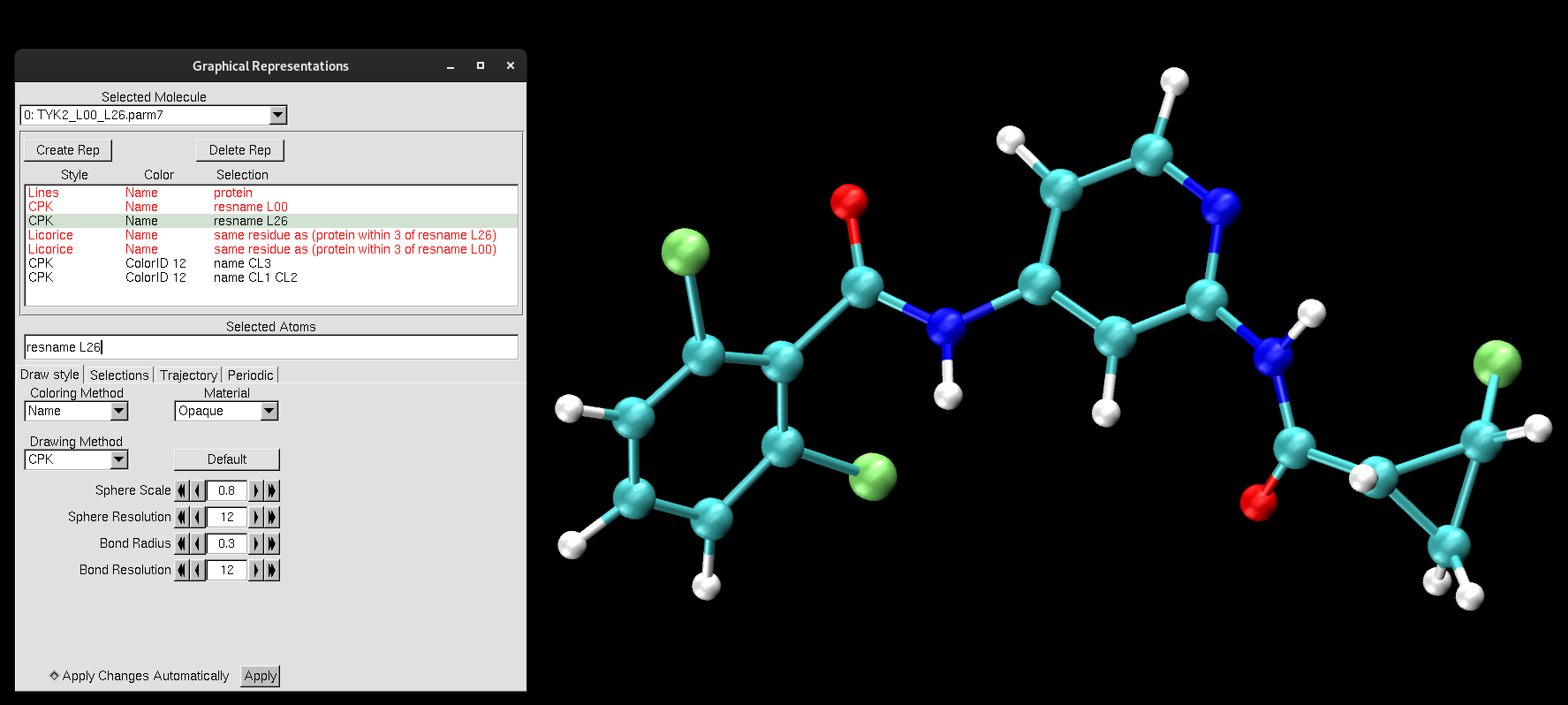
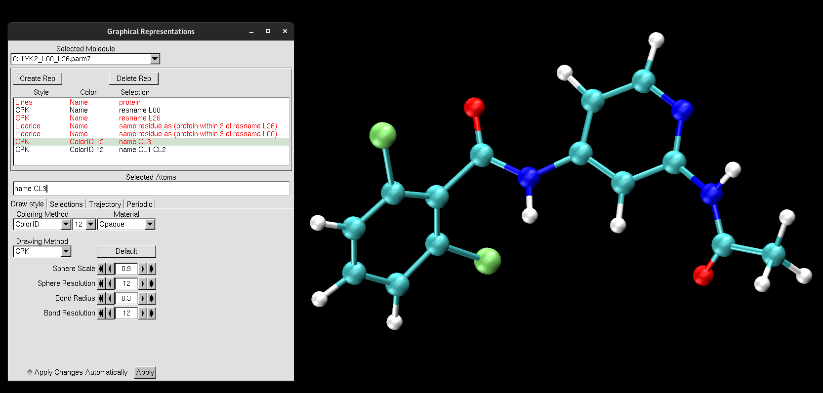
Now, you are going to make use of those special keywords to observe variance in the number of hydrogen-bonding contacts between the ligands and the protein. Hydrogen bonding has the potential to be a factor in the binding affinity.

The selection in parentheses "protein within 3 of resname L26" will select the atoms that are within that distance. 3 Å is an appropriate distance cutoff to highlight potential hydrogen-bonding contacts. Based on the selection within the parentheses, the "same residue as" will select the entire residue that the selection in parentheses belongs to. Moreover, if you were to just type the selection within the parenthesis, you would see that only the atoms (not entire residues) of the protein that are within 3 Å of ligand L26 pop up. The same keyword will select the entire residue that pops up from that selection.Parentheses and keywords allow for flexible and efficient selections.

You should notice that both ligands share the same number of hydrogen bonding contacts, VAL94.

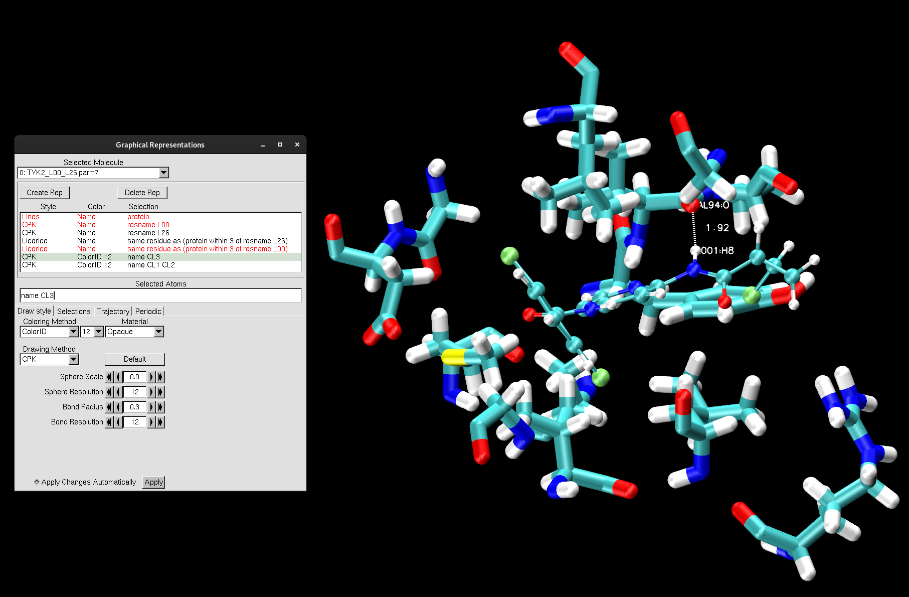
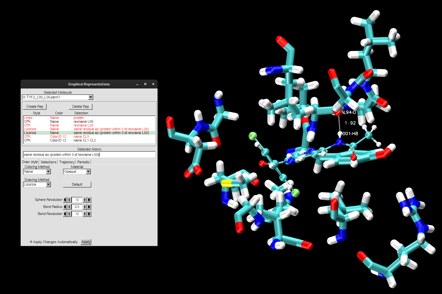
You will now look at the animation of the trajectory to see if you can determine which ligand is the "dummy atom" in this endstate1_.nc trajectory and which ligand is interacting. To do so:

Hint: pay attention to the tail end of the ligand (where the L26 is different from L00).

After watching each ligand throughout the trajectory, can you determine which ligand is the "dummy atom", i.e., which ligand is non-interacting in endstate1?

1.7 Calculating Root-Mean-Square Deviation (RMSD)

Now, you will learn how to use VMD to calculate an RMSD. This time instead of loading a PDB file, you will now load a trajectory file of the MTR1 system. The trajectory is from an AMBER MD simulation, and this system will be used in the additional tutorials. In the directory /expanse/projects/qstore/amber_ws/tutorials/VMD_CPPTRAJ_Basics/input_files/MTR1, you will see the files obtained from MD simulations of the RNA enzyme system, MTR1. The files are MTR1_prot-run.parm7 and centered.MTR1_prot-run.nc (or with .dcd extension).

To open the trajectory of MTR1 in the current session, you can follow the steps we took before to loading a system:

If you are using the terminal to load a new VMD session:

[user@expanse] vmd MTR1_prot-run.parm7 centered.MTR1_prot-run.nc

*Larger trajectories will take longer to load into VMD.

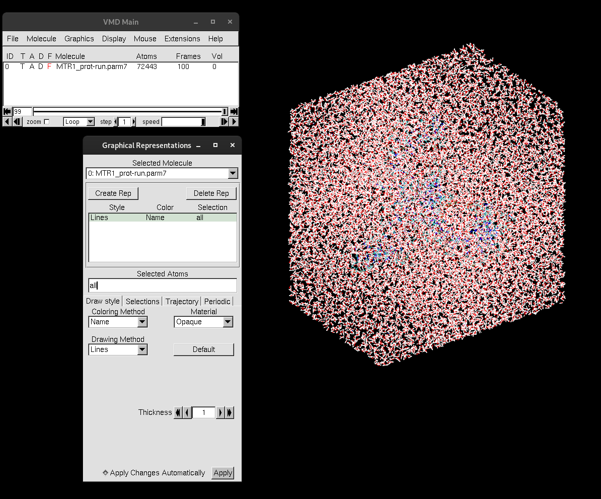
If you decided to load both systems into one VMD session, you will now see in VMD Main that there are multiple molecules loaded.

With a trajectory now loaded, you can now make use of the animation toolbar at the bottom in VMD Main. The slider will transition through the frames, with the number to the left of the slider indicating which frame you are viewing. You can also play the trajectory as an animation, change the speed of the animation and change the animation type (ex: Loop).

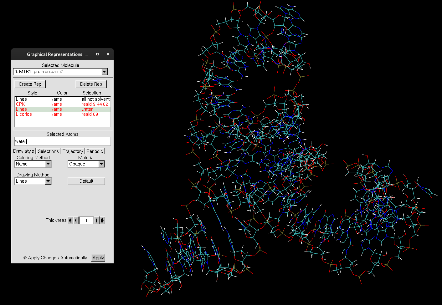
To get started with our MTR1 trajectory analysis, create the following representations:

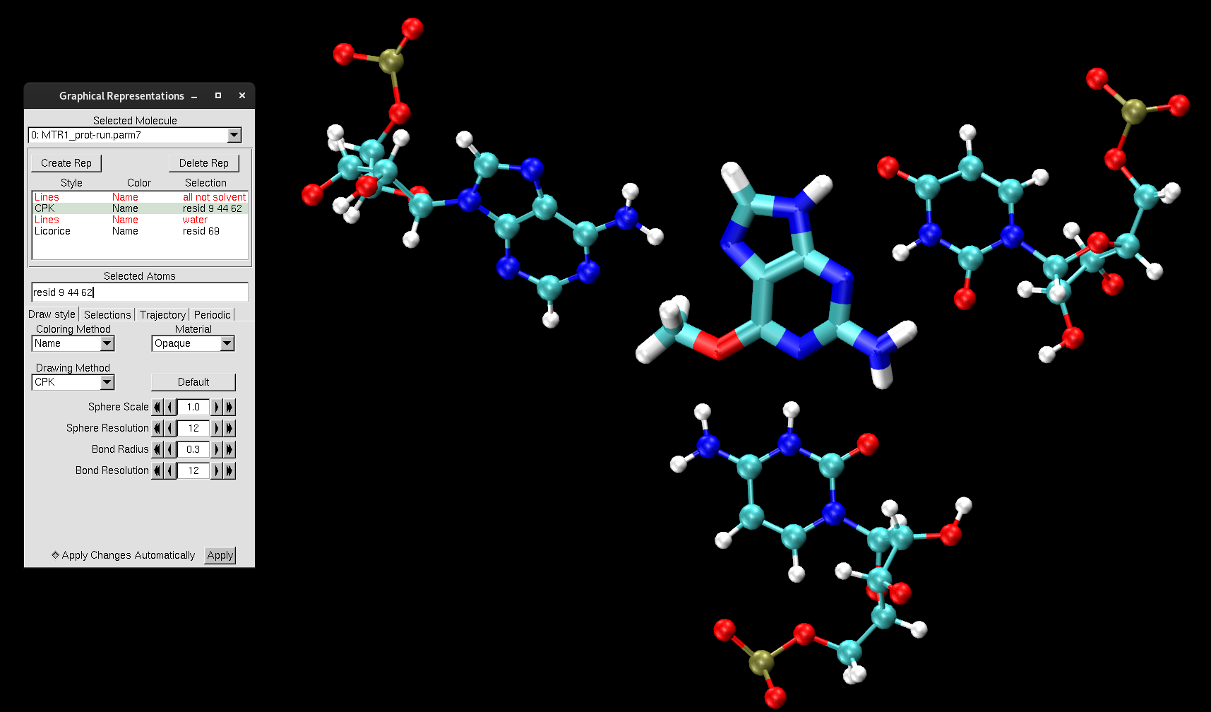
As mentioned before, we will use VMD to calculate its Root Mean Square Deviation (RMSD). RMSDs are helpful in understanding how much the structure deviates from the original starting structure over the time of the simulation. This is an important metric to support if you have a stable structure or not.

To perform this analysis:

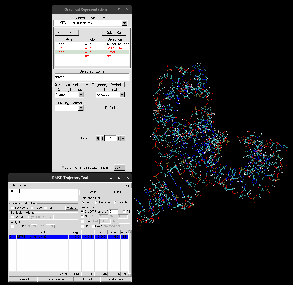
Access the RMSD Trajectory Tool by going to:

You can be more specific with your selection for an RMSD calculation, such as, typing "resid 9 44 62 69". The tick boxes you see allows for quicker selections to add on:

Once you made your selection:

You might see a shift in the structure, that is VMD aligning the molecule to your selection ("nucleic") from frame 1. If you have multiple structures loaded, you will see them in the table within the RMSD Trajectory Tool window. If this were the case, you decide which structure is the Reference mol and which structures to align to that. You do not need to worry too much about that now.

It is important to note aligning with Align should be a step that you do to set up a polished version of the trajectory for visualization. If you do not align your molecule throughout the frames in your trajectory, the structure will jump all around as it switches frames, making it impossible to get a grasp on things.

After you have hit the Align button:

The RMSD values for calculation will print in the table, including the average RMSD and the standard deviation.

To gain further insight into the meaning of the RMSD:

The plot generated depicts the RMSD (in Å) with each frame of the trajectory. This plot provides valuable insights into the movement of your selection. High RMSD values should be noted, as that indicates that the molecule is undergoing significant structural changes. If the RMSD continues to climb, this is indicative of the structure either failing to reach equilibrium or that there is instability in the structure. If this were to be the case for you, it is suggested that you narrow down your selection to try and investigate which regions are responsible for the most change. In general, RMSDs tend to climb throughout the beginning of simulation, but there is a period in which it stabilizes. You must have a stable structure to depart from for further computation exploration.

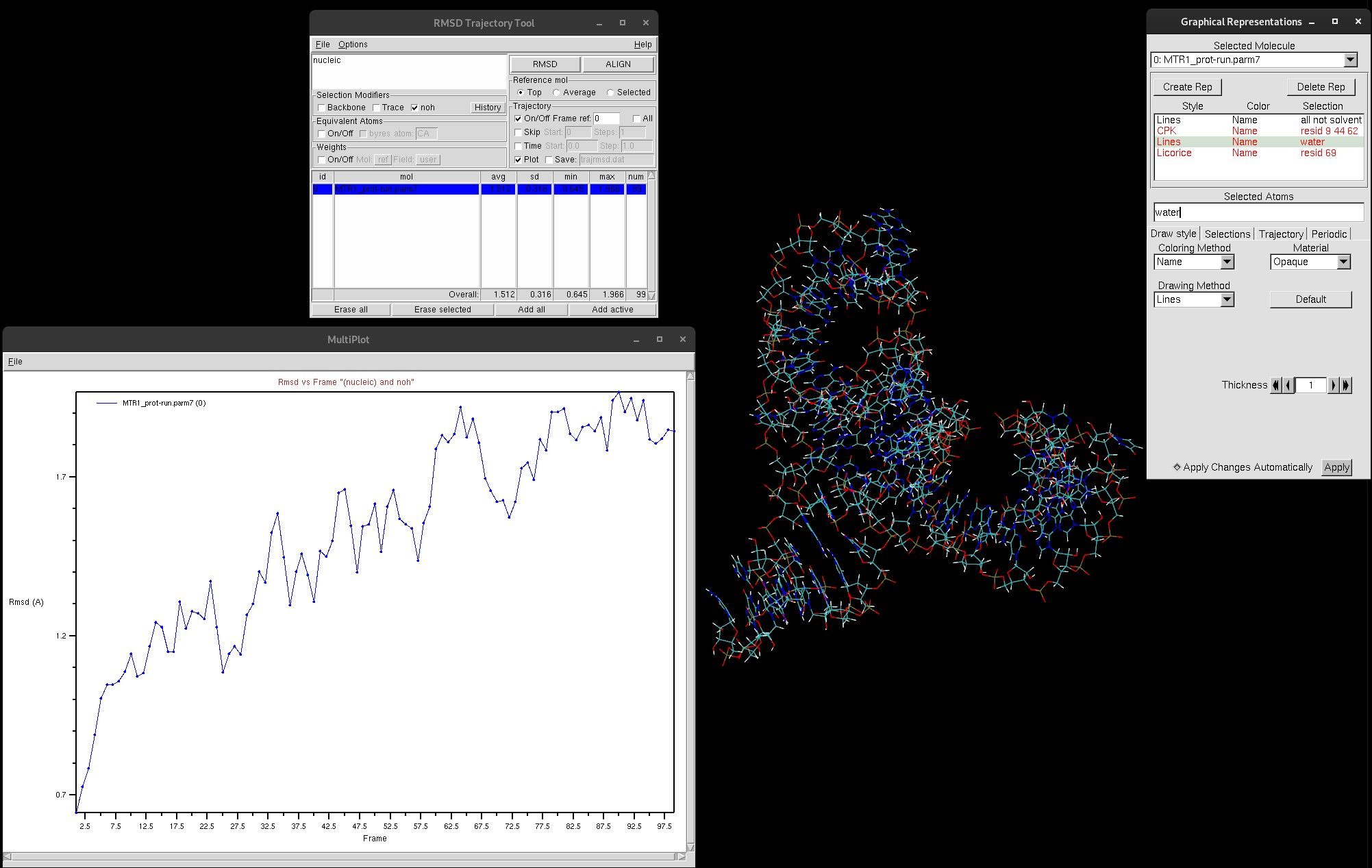
As you can see, the RMSD is trending upwards, however, if you look at the value of Å, the RMSD is very low. This indicates the structure is quite stable.

1.8 Image Rendering

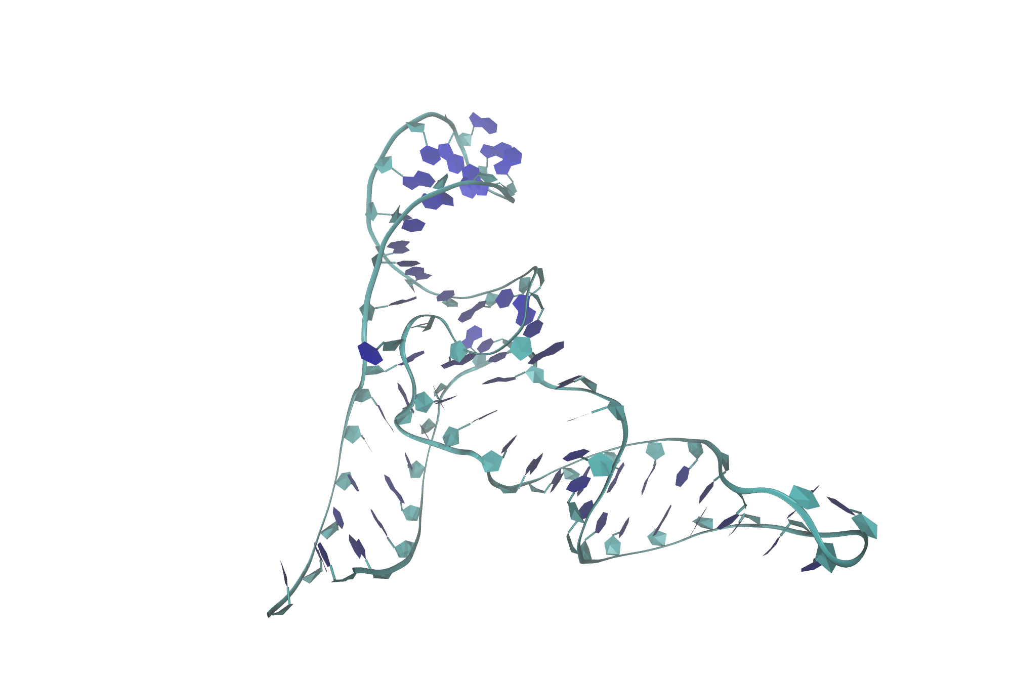
Another tool of VMD is to render high-quality images and animations of your system for posters, presentations or publications. We will quickly walk through the steps to obtain a high-quality image on this MTR1 system. First you must set up the scene that you want to display for your high-quality image.

Next, you can change the projection mode:

VMD offers two projection modes including Perspective and Orthographic. The Perspective mode shows the structure with perspective, meaning objects further from the viewer appear smaller than those closer. This mode is useful for generating images. The Orthographic mode provides a uniform scale across the entire image, which is useful for trajectory analysis.

You can also turn the Depth Cueing on or off by:

This option provides a realistic 3D view with depth perception.

You can change the background color to white through:

Now, once you have the display to your liking, render the image by going to:

In the pop-up window, the default program used to render the image is "Snapshot (VMD OpenGL window)”. This is low quality and not recommended for obtaining high-quality images. In the drop-down menu:

Your high-quality image will pop up! If it is not to your liking, feel free to change the settings, adjust the view and render again.

2.1 Introduction to CPPTRAJ

CPPTRAJ is a valuable asset to complement your computational toolkit, as this AMBER program can be used to achieve a more complex analysis of MD trajectories. In this section, you will learn how to use CPPTRAJ to wrap trajectories, provide the distribution of the degree of angle of a trajectory, calculate RMSDs/RMSFs, and find an average structure from a trajectory.

For this tutorial, you will be given multiple CPPTRAJ input files. Each input file contains lines of commands for CPPTRAJ, but they can each be individually submitted in the interactive command line of CPPTRAJ. The interactive command line of CPPTRAJ can be accessed by typing into your terminal:

[user@expanse] cpptraj

Which will open up the interactive command line seen below:

[user@expanse] cpptraj
CPPTRAJ: Trajectory Analysis. V4.26.4 (AmberTools V20.00)
  ___  ___  ___  ___
   | \/ | \/ | \/ |
  _|_/\_|_/\_|_/\_|_




| Date/time: 00/00/24 00:00:00
| Available memory: 54.268 GB

2.2 Wrapping Trajectories

In this section, you will explore acetic acid in solution and acid acid in the gas phase. Your goal is to understand how the dihedral angle behaves in each environment. However, before you start the analysis on the trajectories of each system, you must first wrap the systems. Wrapping a trajectory means adjusting the positions of the molecules in a simulation so that they can stay within your defined simulation box. Without wrapping a trajectory, visually the molecules within the system can appear to look separated, drifting away or blown out due to the periodic boundary conditions. Therefore, it can be hard to gain an accurate interpretation of what is true behavior displayed in your system. If you are wanting to visually inspect your system, wrapping should be the first step prior to trajectory analysis to avoid confusion. Wrapping is one of CPPTRAJ's most essential roles.

CPPTRAJ can wrap both restart files and trajectory files. In this case, you will be wrapping the trajectory file of acetic acid in solution. First, you must decide on a center in which to wrap everything around. Usually, this is the ligand. Therefore, in this tutorial, it will be ligand L01 (acetic acid). Let's start with the acetic acid in the gas phase trajectory first.

[user@expanse] cpptraj

Similarly to VMD, you must load the topology file first, followed by the trajectory file. CPPTRAJ's command to load a topology file is parm.

> parm acetic_acid_aq.parm7

Then, load the trajectory file with the trajin command. Windows Users: load DCD trajectory file.

> trajin acetic_acid_aq.nc

Next, the command reference is used to tell CPPTRAJ to use a specified set of coordinates to be the reference structure. It is good practice for the reference structure to be wrapped and centered itself.

> reference centered.acetic_acid_aq.rst7

> center :L01 mass

The atom selection is the atom(s)/molecule that we are wanting to be the center. The mask :L01 specifies all the atoms in residue L01. mass indicates that the centering should be done based on the center of mass of the atom selection. Lastly, reference tells cpptraj that the centering should be related to the reference structure that has previously been loaded.

> autoimage :L01 

> center :L01 reference

> trajout centered.acetic_acid_aq.nc

Once you have entered all of that:

> run

> quit

Your interactive terminal of CPPTRAJ should look like this:

[user@expanse] cpptraj
 > parm acetic_acid_aq.parm7
 [parm acetic_acid_aq.parm7]
 Reading 'acetic_acid_aq.parm7' as Amber Topology
 Radius Set: modified Bondi radii (mbondi)
> trajin acetic_acid_aq.nc
 [trajin acetic_acid_aq.nc]
 Reading 'acetic_acid_aq.nc' as Amber NetCDF
> reference centered.acetic_acid_aq.rst7
 [reference centered.acetic_acid_aq.rst7]
 Reading 'centered.acetic_acid_aq.rst7' as Amber Restart
 Setting active reference for distance-based masks: 'centered.acetic_acid_aq.rst7'
> center :L01 mass
 [center :L01 mass]
   CENTER: Centering coordinates using center of mass of atoms in mask (:L01) to
 box center.
> autoimage :L01
 [autoimage :L01]
   AUTOIMAGE: To box center based on center of mass, anchor mask is [:L01]
> center :L01 mass reference
 [center :L01 mass reference]
   CENTER: Centering coordinates using center of mass of atoms in mask (:L01) to
 center of mask (:L01) in reference 'centered.acetic_acid_aq.rst7'.
> trajout centered.acetic_acid_aq.nc
 [trajout centered.acetic_acid_aq.nc]
 Writing 'centered.acetic_acid_aq.nc' as Amber NetCDF
> run
 [run]
---------- RUN BEGIN -------------------------------------------------


PARAMETER FILES (1 total):
0: acetic_acid_aq.parm7, 11740 atoms, 2946 res, box: Orthogonal, 2946 mol, 2929 solvent


INPUT TRAJECTORIES (1 total):
0: 'acetic_acid_aq.nc' is a NetCDF AMBER trajectory with coordinates, velocities, time, box, Parm acetic_acid_aq.parm7 (Orthogonal box) (reading 21 of 21)
 Coordinate processing will occur on 21 frames.


REFERENCE FRAMES (1 total):
   0: centered.acetic_acid_aq.rst7:1
 Active reference frame for distance-based masks is 'Cpptraj Generated Restart'


OUTPUT TRAJECTORIES (1 total):
 'centered.acetic_acid_aq.nc' (21 frames) is a NetCDF AMBER trajectory


BEGIN TRAJECTORY PROCESSING:
.....................................................
ACTION SETUP FOR PARM 'acetic_acid_aq.parm7' (3 actions):
 0: [center :L01 mass]
 Mask [:L01] corresponds to 8 atoms.
 1: [autoimage :L01]
 Anchoring on atoms selected by mask ':L01'
 Mask [:L01] corresponds to 8 atoms.
 Mask [:L01] corresponds to molecule 1
 2945 molecules are mobile.
 2: [center :L01 mass reference]
 Mask [:L01] corresponds to 8 atoms.
.....................................................
ACTIVE OUTPUT TRAJECTORIES (1):
 centered.acetic_acid_aq.nc (coordinates, velocities, time, box)
----- acetic_acid_aq.nc (1-21, 1) -----
0% 10% 20% 30% 40% 50% 60% 70% 80% 90% 100% Complete.


Read 21 frames and processed 21 frames.
TIME: Avg. throughput= 202.0474 frames / second.


ACTION OUTPUT:
TIME: Analyses took 0.0000 seconds.


RUN TIMING:
TIME:   Init               : 0.0001 s (  0.14%)
TIME:   Trajectory Process : 0.1039 s ( 98.88%)
TIME:   Action Post        : 0.0000 s (  0.00%)
TIME:   Analysis           : 0.0000 s (  0.00%)
TIME:   Data File Write    : 0.0000 s (  0.00%)
TIME:   Other              : 0.0010 s (  0.01%)
TIME: Run Total 0.1051 s
---------- RUN END ---------------------------------------------------
> quit
 [quit]
--------------------------------------------------------------------------------
To cite CPPTRAJ use:
Daniel R. Roe and Thomas E. Cheatham, III, "PTRAJ and CPPTRAJ: Software for
 Processing and Analysis of Molecular Dynamics Trajectory Data". J. Chem.
 Theory Comput., 2013, 9 (7), pp 3084-3095.

The wrapped trajectory is now called centered.acetic_acid_aq.nc.

[user@expanse] cpptraj -i ctraj.wrap_traj_acetic_acid_aq.in

Windows Users: As previously mentioned, Windows does not support the NetCDF plugin for VMD, and the proper DCD trajectory file was provided for you. Here, you can practice converting NetCDF files to DCD files yourself by running the bash script nc2dcd.sh. This file creates ctraj.convert_nc_dcd.in and submits it to CPPTRAJ. The file contains:

#! /bin/bash
  
  # Define the script name
  thisScript='basename "$0"'
  
  # Check if the number of arguments is exactly 2
  if ! [ "$#" -eq 2 ]; then
    cat <<EOF
  Needs two file names:
  $thisScript [parm].parm7 [traj].nc
  EOF
    exit 0
  fi
  
  # Load the appropriate module files
  module purge
  module load workshop/amber24
  
  # Define arguments
  parm_file=$1
  traj_file=$2
  
  # Remove the .nc extension
  if [[ $traj_file == *.nc ]]; then
      traj_base=${traj_file%.nc}
  else
      traj_base=$traj_file
  fi
  
  # Create CPPTRAJ input file
  cat <<EOF > ctraj.convert_nc_dcd.in
  parm ${parm_file}
  trajin ${traj_base}.nc
  trajout ${traj_base}.dcd
  run
  quit
  EOF
  
  # Submit the CPPTRAJ input file
  cpptraj -i ctraj.convert_nc_dcd.in > c.log
  rm c.log

This script needs to be fed two arguments to run: the first is the topology file and the second is NetCDF trajectory file.

[user@expanse] bash nc2dcd.sh acetic_acid_vac.parm7 centered.acetic_acid_vac.nc

You should now see in your directory centered.acetic_acid_vac.dcd and the CPPTRAJ input file, ctraj.convert_nc_dcd.in, that was created and submitted.

2.3 Trajectory Time Series and Distribution Analysis

Early on in this tutorial, you measured a dihedral angle of a static structure of acetic acid in solution using VMD. You will be examining the same dihedral angle of the acetic acid molecule when it is in the gas phase and when it is in solution. The aim of this section is to track the movement of the hydrogen in the hydroxyl group throughout each of the trajectories. Furthermore, you will be introduced to xmgrace in order to create a graph comparing the degree of the dihedral angle in different environments.

The xmgrace module on Expanse conflicts with AMBER on Expanse. Therefore, it is recommended to open another Expanse window, To load the xmgrace module, you will need to load:

[user@expanse] module load cpu/0.15.4 intel/19.1.1.217 grace/5.1.25

Then load the xmgrace module:

[user@expanse] module load grace

To access xmgrace, use:

[user@expanse] xmgrace

The script that you will submit CPPTRAJ for acetic acid in gas is called ctraj.dihedral_vac.in and looks like this:

parm acetic_acid_vac.parm7
trajin centered.acetic_acid_vac.nc
dihedral :L01@H4 :L01@O2 :L01@C2 :L01@C1 out dihedral_acetic_acid_vac.dat
run
quit

The submit script for acetic acid in solution, ctraj.dihedral_aq.in, is:

parm acetic_acid_aq.parm7
trajin centered.acetic_acid_aq.nc
dihedral :L01@H4 :L01@O2 :L01@C2 :L01@C1 out dihedral_acetic_acid_aq.dat
run
quit

Submit each input file one at a time, via the command line in your terminal:

[user@expanse] cpptraj -i ctraj.dihedral_vac.in

[user@expanse] cpptraj -i ctraj.dihedral_aq.in

Look for the two files dihedral_acetic_acid_vac.dat and dihedral_acetic_acid_aq.dat. You will use a common graphing program called xmgrace to open these files.

To do so, type:

[user@expanse]xmgrace dihedral_acetic_acid_vac.dat dihedral_acetic_acid_aq.dat

Which will bring up the following:

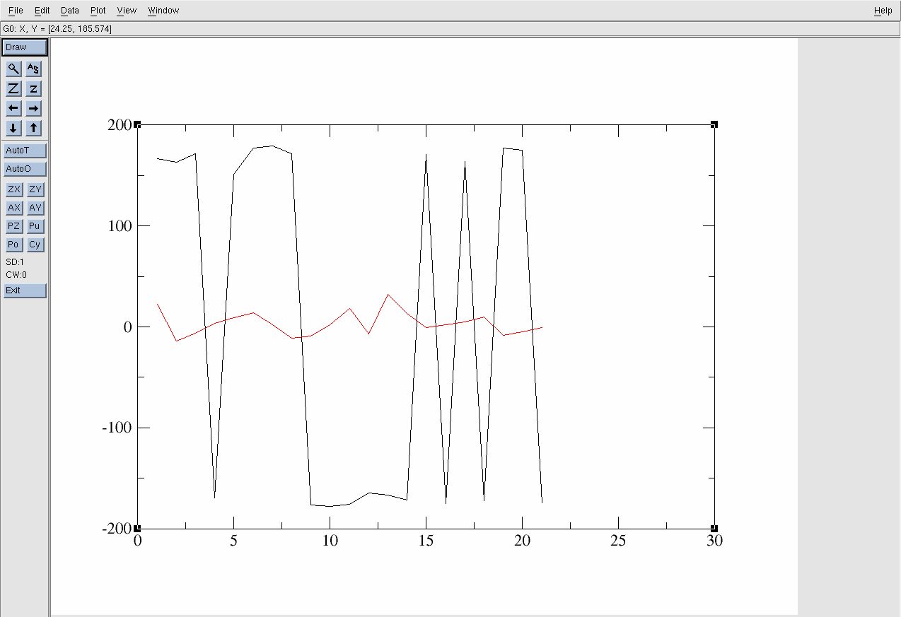
The black line is the acetic acid molecule in the gas phase and the red line is it in the solution environment. The x-axis is the Frame and the y-axis is the degree of the Dihedral angle.

However, the current range of the y-axis (-200 to 200) hinders an intuitive understanding of the dihedral angle fluctuation. Therefore, it is necessary to transform the data to be in the range of -90° to +270°. To achieve this:

Go to Data→Transformations→Evaluate Expression.

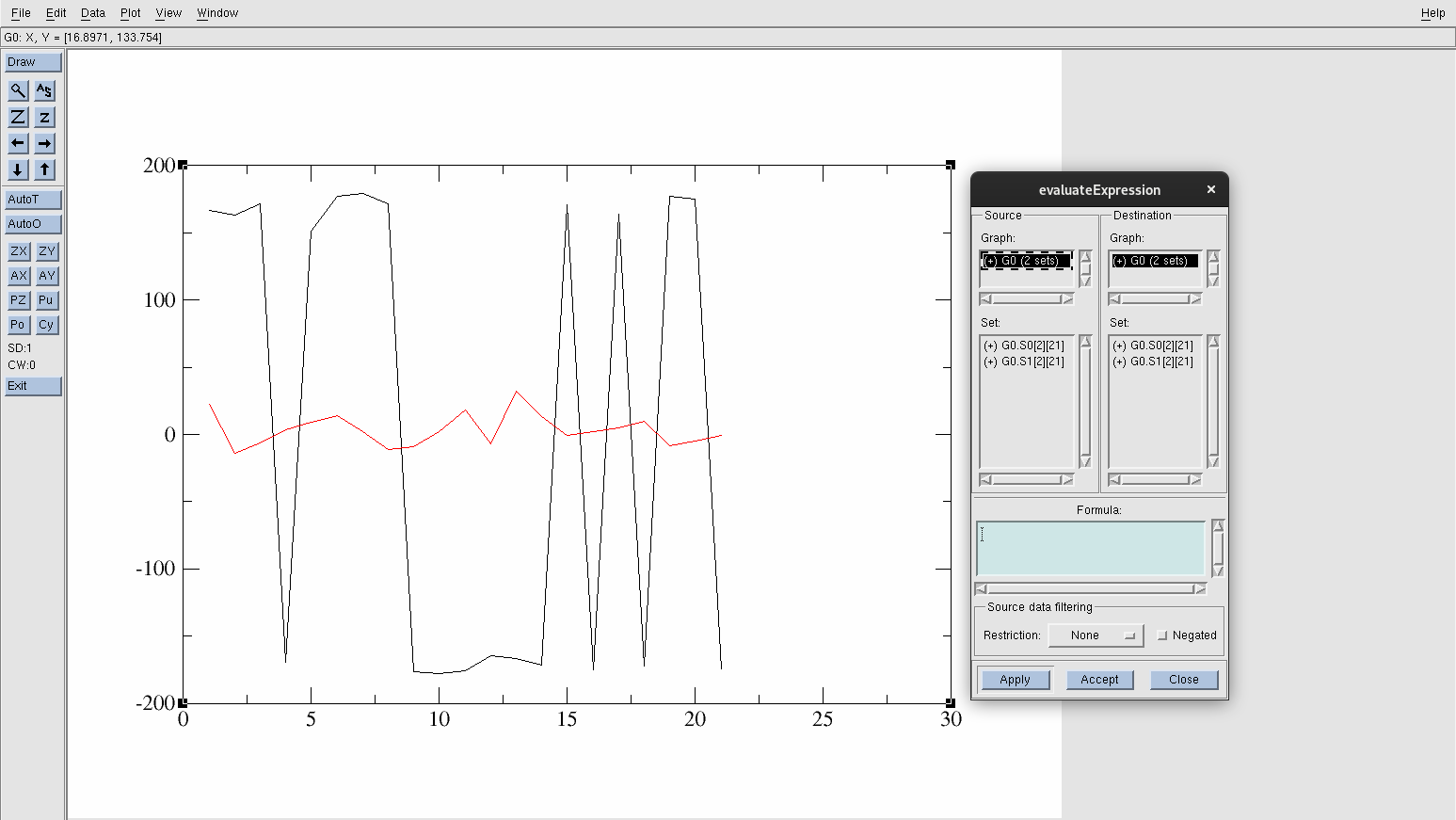
Conveniently in xmgrace, you can easily manipulate your data. To transform the y-values to be within the range -90° to +270°:

Find and select G0.S0[2][21]. (This is the acetic acid in the gas phase data set and will be highlighted in black when selected).

In the Formula section, type the following: y=(y+360) % 360.

Press Apply.

This will produce a new data set called G0.S2[2][21] graphed in a green line:

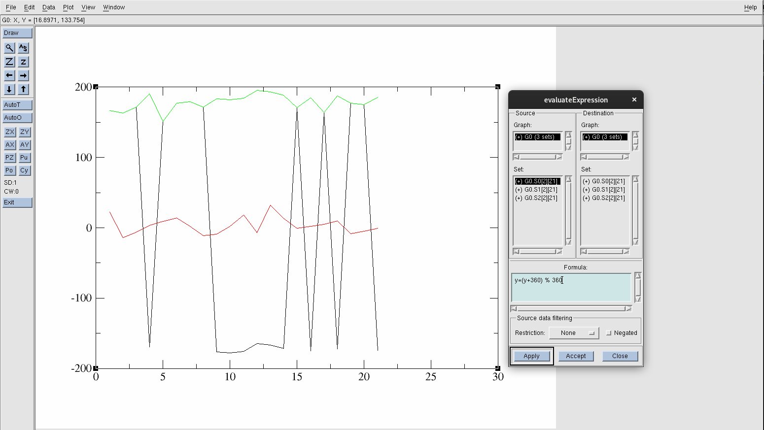
This formula shifts the y-values by 360° to bring all the negative angles into a positive range. The % 360 operation ensures that the new values will be within the 0 to 360 range. If any of the angles exceed 360°, they are wrapped. For example, 370° would become 10°.

Hide the original data set by going to Plot→Set Appearance.

Find and select G0.S0[2][21]. Right-click and choose Hide. You know it will be hidden if the (+) in front of the data set changes to (-).

Select G0.S1[2][21] and increase the width under Line Properties to 2.5.

Hit Apply.

Select G0.S2[2][21] and increase the width under Line Properties to 2.5.

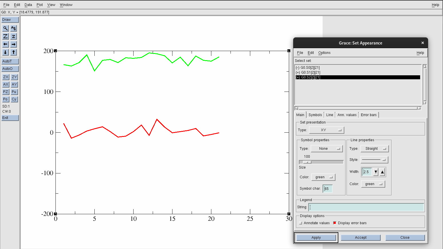
The AS button on the left-side panel of Xmgrace will always adjust the axis automatically for you.

Press the AS button. You should now only see a green line (acid acid in gas with transformed y-values) and a red line (acetic acid in solution)

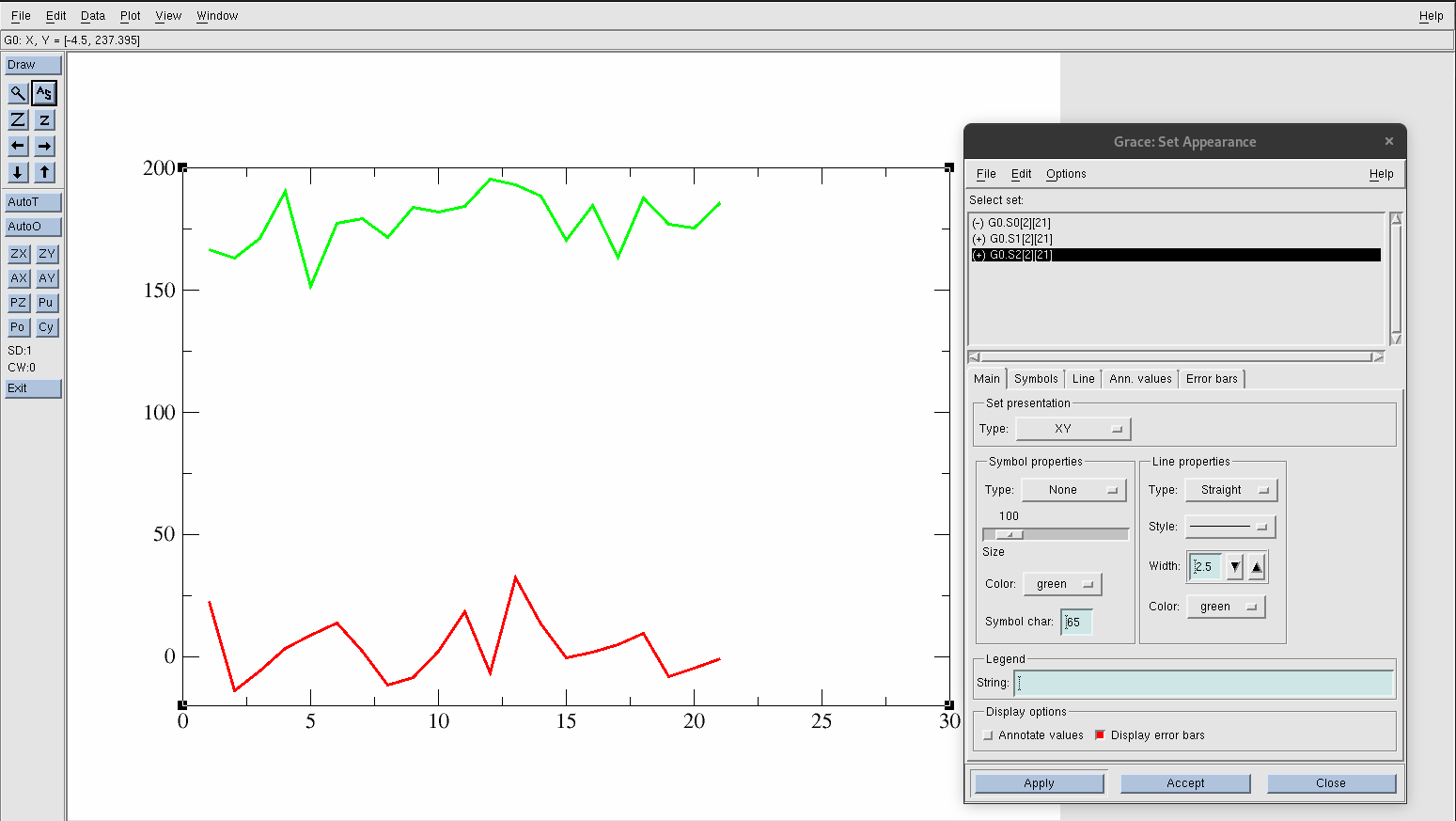
The x-axis is the number of frames, while the y-axis is the dihedral angle in °. To change the range of the axes:

Go to Plot→Axis Properties.

The Edit: should read X axis.

Find the Start and Stop boxes.

Change the Start to 1.

Change the Stop to 21.

Press Apply.

To label the axes:

Find Label String.

Type Frame.

Press Apply.

To change the axis label and values of the y-axis:

Select Y axis from Edit:.

Find the Start and Stop boxes.

Change the Start to -90.

Change the Stop to 270.

Press Apply.

To label the axes:

Find Label String.

Type Dihedral (\c0\C).

Press Apply.

Save this graph by:

Go to File→Save As.

Save the file as acetic_acid_frameVSdihedral.agr

To save the graph as a PNG file type:

Go to File→Print Setup.

Under Device setup, change the PostScript to PNG.

Then, under Page, find the Dimensions line.

Click pix, and change to in.

Change the Resolution to 300.

Hit Apply.

Go back to File and click on Print.

Your graph should look like:

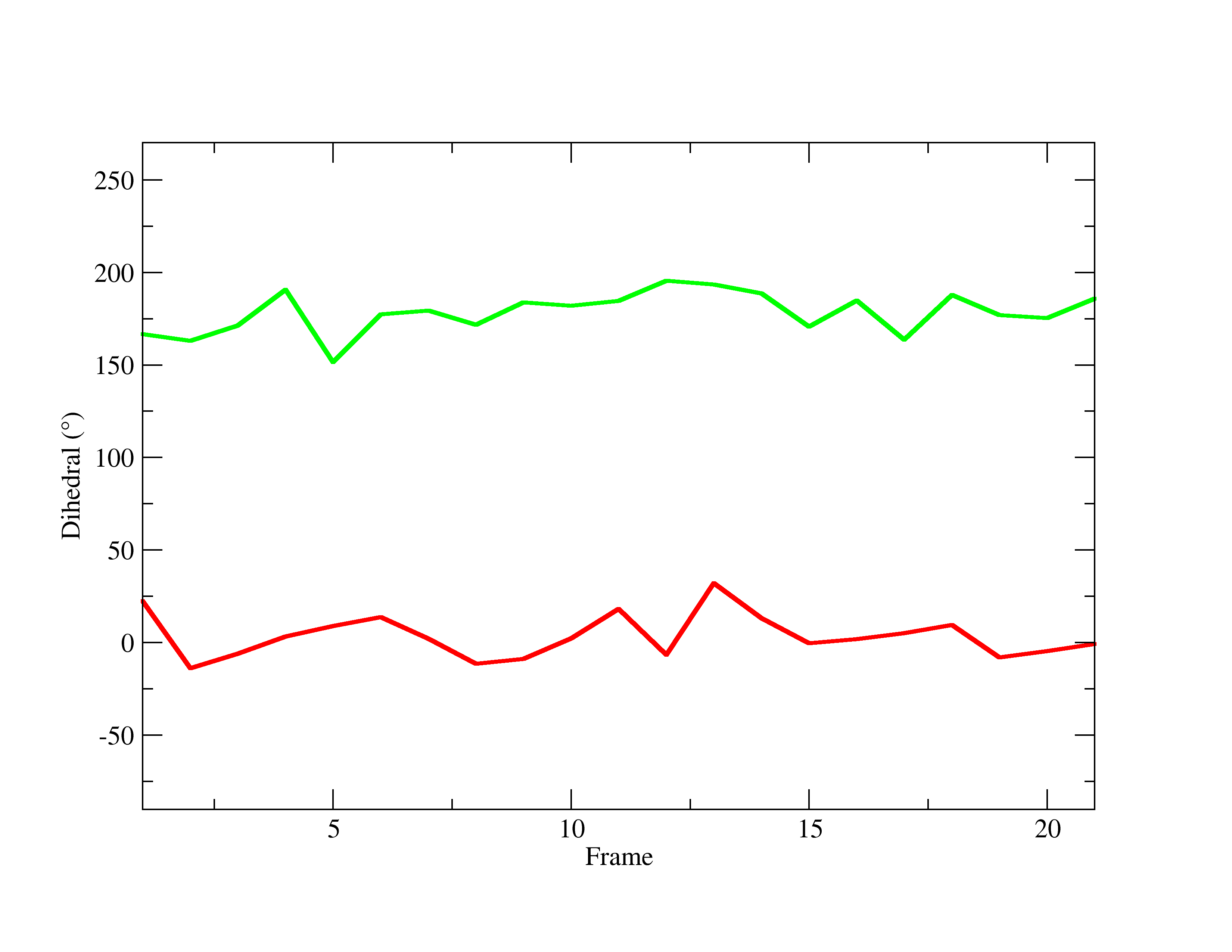
As you can see from the graph, the H4 in the hydroxyl group behaves differently in each environment, fluctuating within a different angle range. To obtain a more meaningful analysis, create a histogram to see the distribution of the data. To do so:

Go to Data→ Transformations→ Histograms.

The window will pop up. Create a histogram for acetic acid in solution first.

Select G0.S1[2][21].

Into Start at: type -15.

Into Stop at: type 35.

Change the # of bins: to 5

Hit Apply.

Select G0.S2[2][21].

Into Start at: type 150.

Into Stop at: type 197.

Change the # of bins: to 5

Hit Apply.

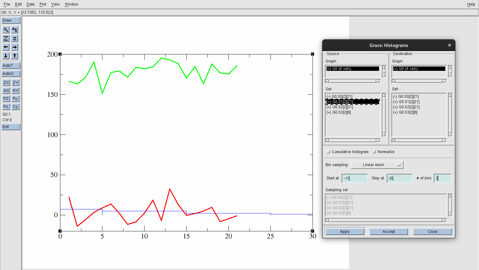
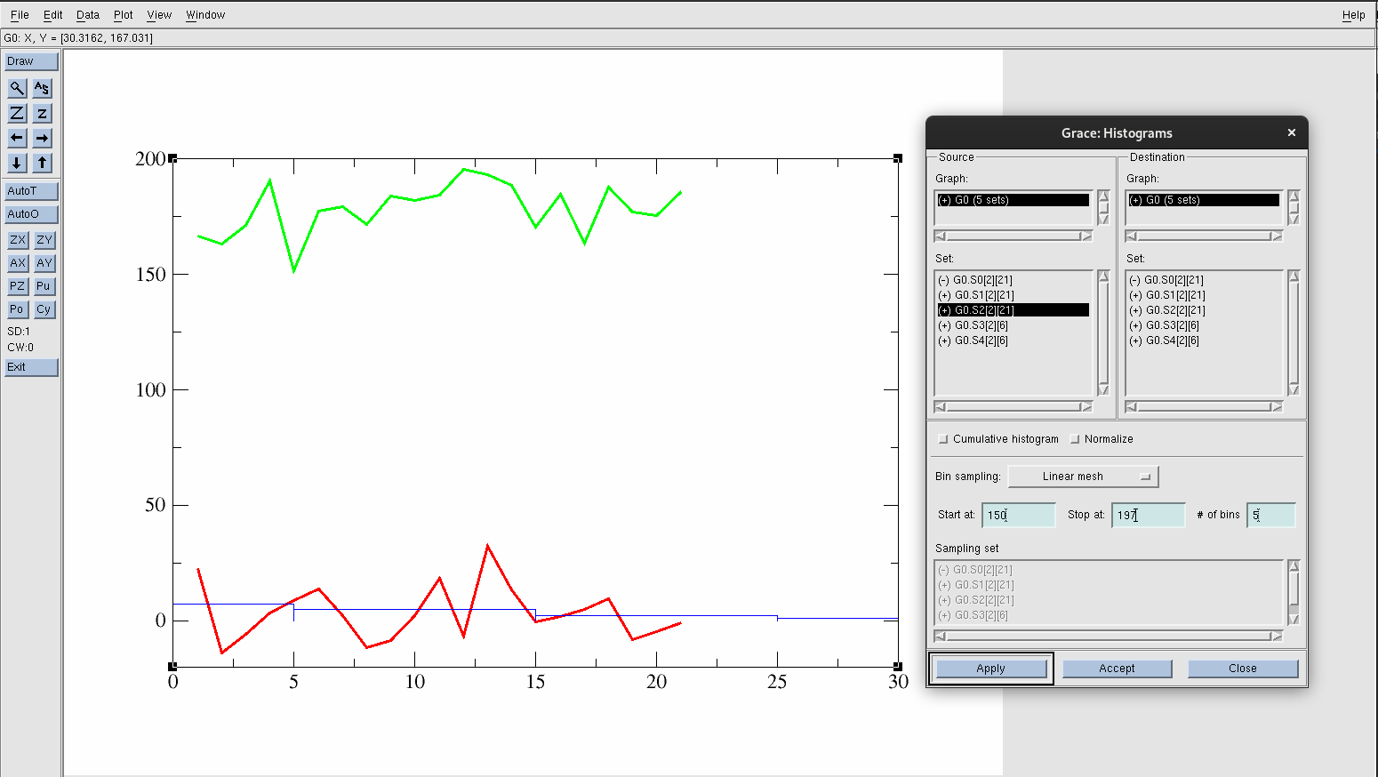
To see the histograms made:

Go back to Plot→Set Appearance.

Hide data set G0.S1[2][21] and G0.S2[2][21].

Press the AS button again.

Select G0.S3[2][21], and change the color to red.

Change the width of the line to 2.5.

Select G0.S4[2][21], and change the color to green.

Change the line width of G0.S4[2][21] to 2.5.

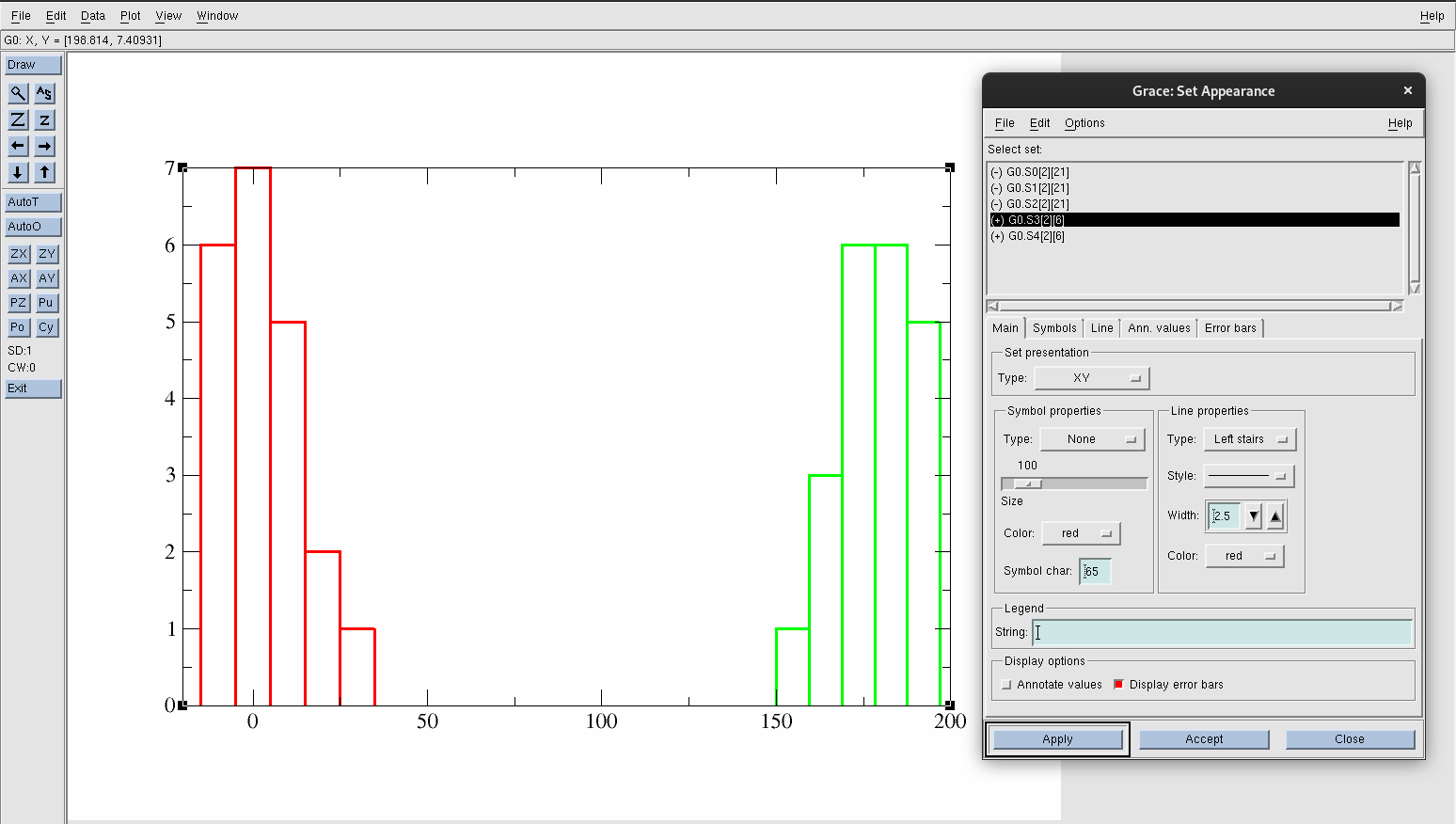
Now, change the axes by again going to:

Plot→Axis Properties.

The Edit: should read X axis.

Find the Start and Stop boxes.

Change the Start to -90.

Change the Stop to 270.

Press Apply.

To label the axes:

Find Label String.

Type Dihedral (\c0\C).

Press Apply.

To change the axis label and values of the y-axis:

Select Y axis from Edit:.

Find the Start and Stop boxes.

Change the Start to 0.

Change the Stop to 10.

Press Apply.

To label the axes:

Find Label String.

Type Frequency.

Press Apply.

Save this graph by:

Go to File→Save As.

Save the file as acetic_acid_dihedral_distru.agr.

To save the graph as a PNG file type:

Go to File→Print Setup.

Under Device setup, change the PostScript to PNG.

Change the file name to match the *.agr file name: acetic_acid_dihedral_distru.png.

Then, under Page, find the Dimensions line.

Click pix, and change to in.

Change the Resolution to 300.

Hit Apply.

Go back to File and click onPrint.

Your graph should look like:

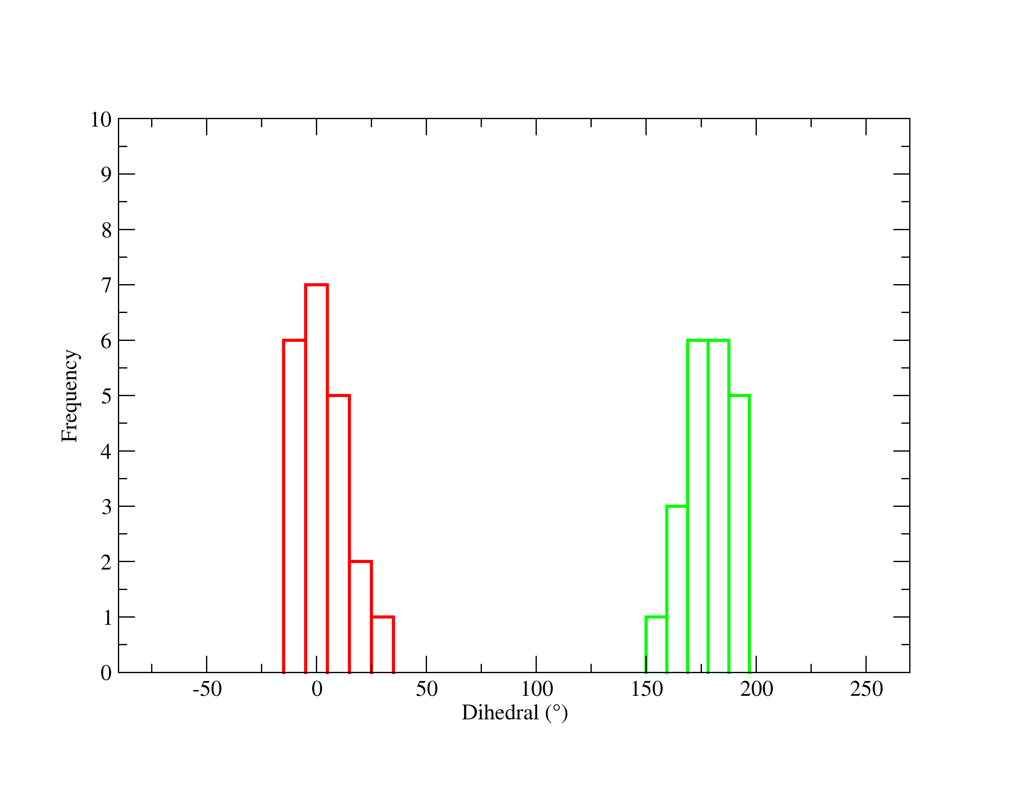
This display is now the distribution graph of the dihedral angles in each system, with the x-agis now as the Dihedral in degrees and the y-axis representing the frequency. The green line is acetic acid in gas and the red line is acetic acid in solution.

Return back to VMD to visually inspect the changes occuring throughout the simulation of the molecule in each system. Visualizing structures is a crucial aspect for MD simulations, as it helps to interpret your numerical data. Furthermore, it is a good practice to constantly look at your structure to ensure that it remains physically realistic and retains your desired properties.

To pull up each of these trajectories in VMD:

Type the following into your teminal, remember, Windows Users will need to load DCD trajectory files:

[user@expanse] vmd -f acetic_acid_vac.parm7 centered.acetic_acid_vac.nc -f acetic_acid_aq.parm7 centered.acetic_acid_aq.nc

This will load each system under one VMD window. The -f flag loads all subsequent files into the same molecule. Meaning, we loaded both systems by first loading the corresponding topology and trajectory file for acetic acid in the gas phase, then the files for acetic acid in solution. Once in VMD, go to Extensions→Analysis→RMSD Trajectory Tool, type resname L01 and then press Align. In your Representations create resname L01 with CPK as the Drawing Method. You should see the acetic acid molecules from each system overlayed on top of each other:

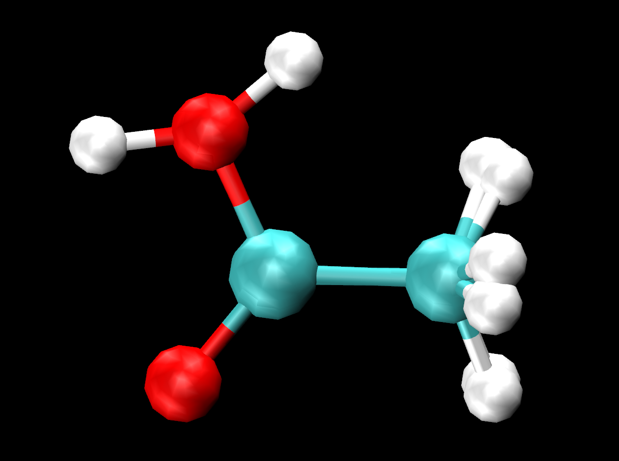
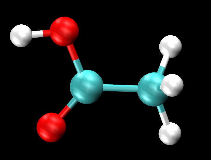
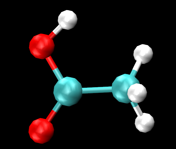
You can turn off one representation at a time to clearly see the difference in orientation of the hydrogen (H4) within the hydroxyl group. You can turn off the representations or in the VMD Main, turn off the display of the acetic acid in solution system completely, (by clicking D) The H4 looks to be making an intramolecular bond with O1 (within the C=O) in the gas phase, but does not show the same in solution. What could be the reasoning behind this change in behavior?

---

2.4 Computing Average Structures and Fluctuations

You have already learned how to create RMSD plots using VMD. With the same system, MTR1, you will now use CPPTRAJ to create RMSDs. Additionally, you will learn how to calculate RMSFs and find the average structure of simulations using CPPTRAJ.

Go to the directory that contains the MTR1 files: /expanse/projects/qstore/amber_ws/tutorials/VMD_CPPTRAJ_Basics/input_files/acetic_acid.

You will find a script called ctraj.RMSD_MTR1.in. The contents of this script is:

parm MTR1_prot-run.parm7
trajin centered.MTR1_prot-run.nc
rms ToFirst :1-69&!@H= first out RMSD_MTR1.dat mass
run
quit

This input file again follows a standard of inputting your topology file first, then your trajectory. The rms ToFirst :1-69&!@H= first out RMSD_MTR1.dat mass line tells cpptraj to do an RMSD calculation, saving the data set as "ToFirst", using all non-hydrogen atoms in the residues 1 through 69. This residue selection is the entire nucleic molecule. The first is telling cpptraj to use the first frame in the trajectory as a reference, with out as the command to write the output to a file named RMSD_MTR1.dat. The mass command indicates a mass-weighted RMSD calculation.

Submit this file as your did before:

[user@expanse] cpptraj -i ctraj.RMSD_MTR1.in

Once the job is complete, the RMSD_MTR1.dat file will be in your directory.

Using xmgrace, open this file:

[user@expanse] xmgrace RMSD_MTR1.dat

Which will pop up:

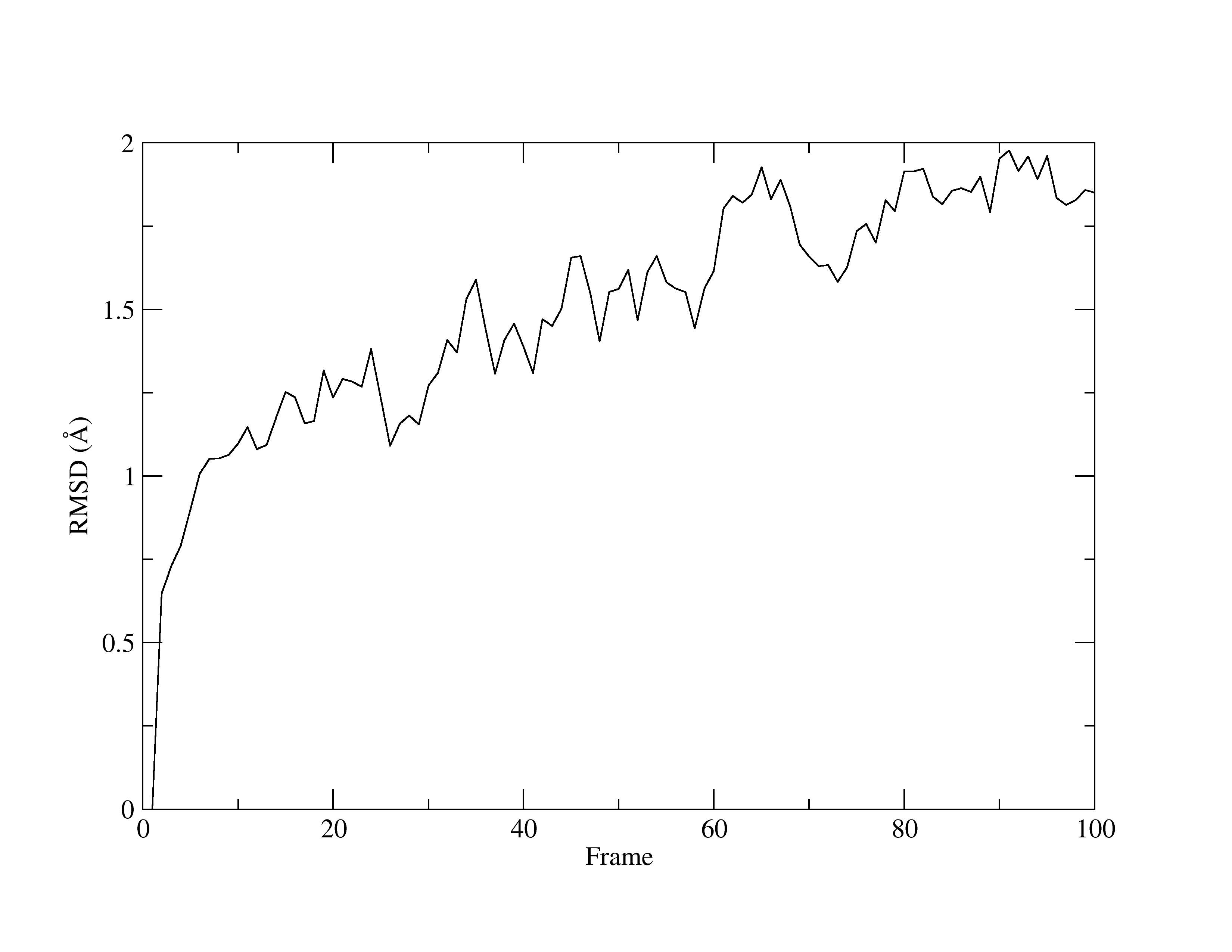
With a quick glance of the graph, you will see that it is comparable to the same graph that was produced by VMD. Once again, the line fluctuates and has an upwards direction. Yet, given the very low values for RMSD, you can concur that the structure is stable.

Next, you will learn to use CPPTRAJ to calculate a Root Mean Square Fluctuation (RMSF). Like RMSDs, RMSFs are important analytical measurements that provide insight into your system. RMSFs quantify the overall flexibility and mobility of each atom or residue within your system as the simulation progresses. RMSFs calculate how much the position of each atom in your selection deviates from its average position throughout the simulation time.

In your directory, find the input file, ctraj.RMSF_MTR1.in.

Open in VIM to see the script:

parm MTR1_prot-run.parm7
reference centered.MTR1_prot-run.rst7
trajin centered.MTR1_prot-run.nc
rms :1-69&!@H reference mass
atomicfluct out RMSF_MTR1.dat :1-69&!@H= byres
atomicfluct out RMSF_Bfact_MTR1.dat :1-69&!@H= byres bfactor
run
quit

The script is similar to the previous one, but there are two new lines containing the RMSF commands.atomicfluct out RMSF.dat :1-69&!@H= byres and atomicfluct out RMSF_Bfact.dat :1-69&!@H= byres bfactor. atomicfluct is the command for an RMSF calculation. As seen before, out directs CPPTRAJ to output the data into a file name of your choosing (here, it is RMSF.dat, followed by your atom selection. The keyword byres specifies the output to be per residue, which sums the fluctuations of all atoms in each residue. The other keyword seen, bfactor, which will calculate the B-factor of the MD trajectory. This is an additional analysis one can do to compare simulation to crystallographic data. A low B-factor is indicative of a well-ordered and stable structure, while a high b-factor suggests more movement and thereby, greater fluctuations.

Open the RMSF.dat by using xmgrace:

[user@expanse] xmgrace RMSF_MTR1.dat

Which will look like this:

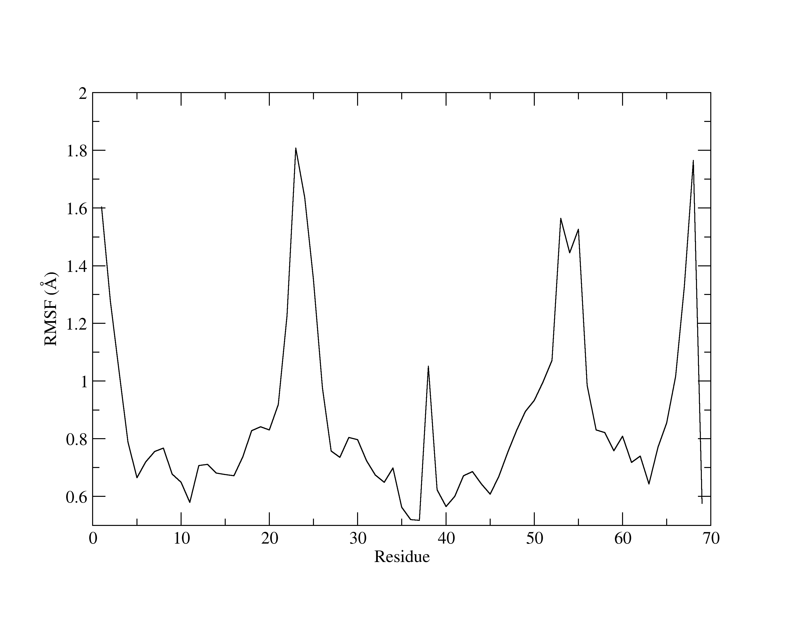
The x-axis is the residue number, while the y-axis shows the fluctuations (in Å). Higher peaks indicate greater fluctuations. RMSFs are useful for identifying residues that have a greater contribution to the overall dynamics of the structure. Usually, it is common for residues involved in crystal contacts to exhibit higher peaks, reflecting increased mobility.

Lastly, you will learn to obtain the average structure of a trajectory using CPPTRAJ with the command average.

Find the input file ctraj.average_MTR1.in and VIM it.

parm MTR1_prot-run.parm7
trajin centered.MTR1_prot-run.nc
average avg.pdb :1-69&!@H= pdb
run
quit

After the average command, you must provide a filename in which to save the data. Here, the name is avg.pdb, followed by the atom selection mask and the file type specification pdb.

Run the input file as usual:

[user@expanse] cpptraj -i ctraj.average_MTR1.in

Now, you have an average structure of MTR1 in a PDB format that can be opened up in VMD for viewing.

---

In this tutorial, you have gained foundational skills in using VMD and CPPTRAJ for visualizing and analyzing trajectories from MD simulations. On the completion of this tutorial, you are ready to proceed to the more advanced AMBER tutorials ahead. Both VMD and CPPTRAJ can be very valuable tools for your studies, so continue to practice and even venture into the more complex analyses that these powerful programs offer.