Erika McCarthy1, Şölen Ekesan1, and Darrin M. York1
1Laboratory for Biomolecular Simulation Research, Institute for Quantitative Biomedicine and Department of Chemistry and Chemical Biology, Rutgers University, Piscataway, NJ 08854, USA
In this tutorial you will learn how to apply a machine learning potential correction (ΔMLP) to semiempirical (DFTB3) simulations and validate the resulting free energy surface using generalized weighted thermodynamic perturbation (gwTP). The tutorial is structured as follows:
The necessary inputs for part 1.1 are available in:
/expanse/projects/qstore/amber_ws/tutorials/MLP-gwTP_MTR1/PBE0_timingtest/inputs
and
/expanse/projects/qstore/amber_ws/tutorials/MLP-gwTP_MTR1/MLP_timingtest/inputs
The subsequent outputs are available in:
/expanse/projects/qstore/amber_ws/tutorials/MLP-gwTP_MTR1/PBE0_timingtest/outputs
and
/expanse/projects/qstore/amber_ws/tutorials/MLP-gwTP_MTR1/MLP_timingtest/outputs
The inputs should be copied to your working directory. If you unable to produce an output for a given step, copy it from the output directory in order to proceed.
[user@cluster] mkdir PBE0_timingtest
[user@cluster] cp -r /expanse/projects/qstore/amber_ws/tutorials/MLP-gwTP_MTR1/PBE0_timingtest/inputs/* ./PBE0_timingtest
[user@cluster] mkdir MLP_timingtest
[user@cluster] cp -r /expanse/projects/qstore/amber_ws/tutorials/MLP-gwTP_MTR1/MLP_timingtest/inputs/* ./MLP_timingtest
Here we will perform a short timing test to demonstrate the speed-up enabled by a ΔMLP compared to an ab initio level calculation. The ΔMLP was trained to correct DFTB3 level energies and forces to replicate PBE0/6-31G* for the MTR1 reaction. First we will run 2 steps of dynamics on a single umbrella window at the PBE0 level using the AMBER interface to QUICK. Simulations using QUICK can be accelerated using a GPU, but in order to stably use comparable electrostatic methods the test will be performed on a CPU. You have been provided img01_PBE0.mdin run_PBE0.slurm, img01.disang, init01.rst7, and a template directory containing the parm file.
PBE0
&cntrl
! IO =======================================
      irest = 0       ! 0 = start, 1 = restart
        ntx = 1       ! 1 = start, 5 = restart
       ntxo = 1       ! read/write rst as formatted file
      iwrap = 1       ! wrap crds to unit cell
     ioutfm = 1       ! write mdcrd as netcdf
       imin = 0
      ntmin = 1
       ntpr = 1
       ntwr = 1
       ntwx = 1
       ntwf = 0
! DYNAMICS =================================
     nstlim = 2    ! number of time steps
         dt = 0.001   ! ps/step
        ntb = 1       ! 1=NVT periodic, 2=NPT periodic, 0=no box
! TEMPERATURE ==============================
      temp0 = 298     ! target temp
   gamma_ln = 5.0     ! Langevin collision freq
        ntt = 3       ! thermostat (3=Langevin)
! PRESSURE  ================================
        ntp = 0       ! 0=no scaling, 1=isotropic, 2=anisotropic
! SHAKE ====================================
        ntc = 2       ! 1=no shake, 2=HX constrained, 3=all constrained
noshakemask = ":69|@272-282,290-291,1975-1988"    ! do not shake these
        ntf = 1       ! 1=cpt all bond E, 2=ignore HX bond E, 3=ignore all bond E
! MISC =====================================
        cut = 10.0
      ifqnt = 1
         ig = -1
     nmropt = 1
/


&wt
type='DUMPFREQ', istep1=1
&end
&wt
  type='END',
&end
DISANG=img01.disang
DUMPAVE=img01.dumpave

&ewald
  dsum_tol = 1.e-6
/

&qmmm
    qm_theory   = 'quick'
        qmmask  = ':69|@272-282,290-291,1975-1988'
      qmcharge  = 1
          spin  = 1
      qmmm_int  = 1
      qm_ewald  = 1
       qmshake  = 0
        itrmax  = 50
       scfconv  = 1e-07
     verbosity  = 0
/

&quick
  method   = 'PBE0'
  basis    = '6-31G*'
/
Note the inclusion of the quick namelist specifying the functional and basis set for the simulation.
[user@cluster] sbatch run_PBE0.slurm You will find that the job takes about 6 minutes to complete. While it runs, let's take a look at the input for the QM/MM+ΔMLP simulation. You have been provided img01_MLP.mdin and run_MLP.slurm. The template directory also contains 4 graph files that each contain a set of machine learning model parameters.
MLP
&cntrl
! IO =======================================
      irest = 0       ! 0 = start, 1 = restart
        ntx = 1       ! 1 = start, 5 = restart
       ntxo = 1       ! read/write rst as formatted file
      iwrap = 1       ! wrap crds to unit cell
     ioutfm = 1       ! write mdcrd as netcdf
       imin = 0
      ntmin = 1
       ntpr = 1
       ntwr = 1
       ntwx = 1
       ntwf = 0
! DYNAMICS =================================
     nstlim = 2       ! number of time steps
         dt = 0.001   ! ps/step
        ntb = 1       ! 1=NVT periodic, 2=NPT periodic, 0=no box
! TEMPERATURE ==============================
      temp0 = 298     ! target temp
   gamma_ln = 5.0     ! Langevin collision freq
        ntt = 3       ! thermostat (3=Langevin)
! PRESSURE  ================================
        ntp = 0       ! 0=no scaling, 1=isotropic, 2=anisotropic
! SHAKE ====================================
        ntc = 2       ! 1=no shake, 2=HX constrained, 3=all constrained
noshakemask = ":69|@272-282,290-291,1975-1988"    ! do not shake these
        ntf = 1       ! 1=cpt all bond E, 2=ignore HX bond E, 3=ignore all bond E
! MISC =====================================
        cut = 10.0
      ifqnt = 1
         ig = -1
     nmropt = 1
/


&ewald
  dsum_tol = 1.e-6
/

&qmmm
    qm_theory   = 'DFTB3'
        qmmask  = ':69|@272-282,290-291,1975-1988'
      qmcharge  = 1
          spin  = 1
       qmshake  = 0
      qm_ewald  = 1
   qmmm_switch  = 1
       scfconv  = 1.e-10
     verbosity  = 0
  tight_p_conv  = 1
  diag_routine  = 0
   pseudo_diag  = 1
  dftb_maxiter  = 100
/

&wt type = 'DUMPFREQ', istep1 = 1, /
&wt type='END' /
DISANG=img01.disang
DUMPAVE=img01.dumpave
LISTOUT=POUT
LISTIN=POUT

&dprc
  idprc=1
  mask=":69|@272-282,290-291,1975-1988"
  rcut = 6.0
  intrafile=""
  interfile(1)="template/graph.000.pb"
/
The dprc namelist indicates that we will be using the interface to DeePMD-Kit to apply a Deep Potential Range Correction model (ie the ΔMLP). Here we will also run 2 steps of dynamics.
[user@cluster] sbatch run_MLP.slurm When the jobs are complete, compare the mdinfo files.
NSTEP =        2   TIME(PS) =       0.002  TEMP(K) =    12.93  PRESS =     0.0
 Etot   =  -1139551.3377  EKtot   =      1488.8508  EPtot      =  -1141040.1886
 BOND   =       548.5419  ANGLE   =      1093.1544  DIHED      =      1635.9114
 1-4 NB =       624.7780  1-4 EEL =     -7539.0600  VDWAALS    =     36590.5463
 EELEC  =   -268485.1838  EHBOND  =         0.0000  RESTRAINT  =         2.6047
 QUICKESCF=   -905511.4815
 EAMBER (non-restraint)  =  -1141042.7932
 Ewald error estimate:   0.1108E-04
 NMR restraints: Bond =    0.000   Angle =     0.000   Torsion =     0.000
               : Gen. Dist. Coord. =     2.605
===============================================================================

| Final Performance Info:
| -----------------------------------------------------
| Average timings for last       1 steps:
|     Elapsed(s) =     119.75 Per Step(ms) =  119753.32
|         ns/day =       0.00   seconds/ns = **********
|
| Average timings for all steps:
|     Elapsed(s) =     348.89 Per Step(ms) =  174444.74
|         ns/day =       0.00   seconds/ns = **********
| ----------------------------------------------------- NSTEP = 2 TIME(PS) = 0.002 TEMP(K) = 12.96 PRESS = 0.0
Etot = -1139551.1318 EKtot = 1492.0009 EPtot = -1141043.1327
BOND = 548.9066 ANGLE = 1092.8042 DIHED = 1635.5829
1-4 NB = 624.7320 1-4 EEL = -7539.0003 VDWAALS = 36587.1481
EELEC = -268484.2609 EHBOND = 0.0000 RESTRAINT = 2.5503
DFTBESCF= -5216.9778
ML = -900294.6180
EAMBER (non-restraint) = -1141045.6830
Ewald error estimate: 0.1211E-01
NMR restraints: Bond = 0.000 Angle = 0.000 Torsion = 0.000
: Gen. Dist. Coord. = 2.550
===============================================================================
| Final Performance Info:
| -----------------------------------------------------
| Average timings for last 1 steps:
| Elapsed(s) = 0.54 Per Step(ms) = 540.10
| ns/day = 0.16 seconds/ns = 540099.98
|
| Average timings for all steps:
| Elapsed(s) = 13.63 Per Step(ms) = 6812.91
| ns/day = 0.01 seconds/ns = 6812913.00
| -----------------------------------------------------In general, the first step of dynamics is always the slowest, so for an accurate comparison, one should look at the timing for the last step. This took 119.75 seconds per step with PBE0 and 0.54 seconds per step with the ΔMLP. The ΔMLP provides a significant speed-up over the ab initio simulation, and as you will demonstrate in the next section, it does so with high accuracy.
Section 1.2 will walk you through a set of simulations that have already been performed. The necessary inputs for those simulations are available in:
/expanse/projects/qstore/amber_ws/tutorials/MLP-gwTP_MTR1/gwTP/input
The subsequent outputs for you to analyze are available in:
/expanse/projects/qstore/amber_ws/tutorials/MLP-gwTP_MTR1/gwTP/output
[user@cluster] mkdir MLP-gwTP
[user@cluster] cd MLP-gwTP
[user@cluster] cp -r /expanse/projects/qstore/amber_ws/tutorials/MLP-gwTP_MTR1/gwTP/output ./
[user@cluster] cd output
Next you will learn how to validate the accuracy of the ΔMLP model using gwTP, but first we will review how the data was generated. These simulations and calculations would take longer than there is time for in this exercise, thus the results have been provided for you. You have been given data in which 3 iterations of the SASM (it08, it09, it10) was performed near the final path, each for 4 trials (000, 001, 002, 003). The 4 trials each apply 1 of the 4 graph files in the template directory when running the simulations. These 4 sets of neural network parameters were generated stochastically when the training was performed using the DeePMD-Kit program. They serve as multiple reference Hamiltonians for gwTP. If one model is deficient in a particular area of the free energy surface, another model will likely perform better, and will thus be favored during reweighting.
As an example, let's focus on the directory it08_000.
[user@cluster] ls it08_000
img01.disang   img04.mdin     img07.rst7     img11.dumpave  img14.mdout    img18.disang   img21.mdin     img24.rst7     img28.dumpave  img31.mdout
img01.dumpave  img04.mdout    img08.disang   img11.mdin     img14.rst7     img18.dumpave  img21.mdout    img25.disang   img28.mdin     img31.rst7
img01.mdin     img04.rst7     img08.dumpave  img11.mdout    img15.disang   img18.mdin     img21.rst7     img25.dumpave  img28.mdout    img32.disang
img01.mdout    img05.disang   img08.mdin     img11.rst7     img15.dumpave  img18.mdout    img22.disang   img25.mdin     img28.rst7     img32.dumpave
img01.rst7     img05.dumpave  img08.mdout    img12.disang   img15.mdin     img18.rst7     img22.dumpave  img25.mdout    img29.disang   img32.mdin
img02.disang   img05.mdin     img08.rst7     img12.dumpave  img15.mdout    img19.disang   img22.mdin     img25.rst7     img29.dumpave  img32.mdout
img02.dumpave  img05.mdout    img09.disang   img12.mdin     img15.rst7     img19.dumpave  img22.mdout    img26.disang   img29.mdin     img32.rst7
img02.mdin     img05.rst7     img09.dumpave  img12.mdout    img16.disang   img19.mdin     img22.rst7     img26.dumpave  img29.mdout    path.micro.pkl
img02.mdout    img06.disang   img09.mdin     img12.rst7     img16.dumpave  img19.mdout    img23.disang   img26.mdin     img29.rst7     path.sims.pkl
img02.rst7     img06.dumpave  img09.mdout    img13.disang   img16.mdin     img19.rst7     img23.dumpave  img26.mdout    img30.disang   pathconv.txt
img03.disang   img06.mdin     img09.rst7     img13.dumpave  img16.mdout    img20.disang   img23.mdin     img26.rst7     img30.dumpave  reanalysis
img03.dumpave  img06.mdout    img10.disang   img13.mdin     img16.rst7     img20.dumpave  img23.mdout    img27.disang   img30.mdin     rem.08.log
img03.mdin     img06.rst7     img10.dumpave  img13.mdout    img17.disang   img20.mdin     img23.rst7     img27.dumpave  img30.mdout    rem.type
img03.mdout    img07.disang   img10.mdin     img13.rst7     img17.dumpave  img20.mdout    img24.disang   img27.mdin     img30.rst7     samplingconv.txt
img03.rst7     img07.dumpave  img10.mdout    img14.disang   img17.mdin     img20.rst7     img24.dumpave  img27.mdout    img31.disang   sims.txt
img04.disang   img07.mdin     img10.rst7     img14.dumpave  img17.mdout    img21.disang   img24.mdin     img27.rst7     img31.dumpave
img04.dumpave  img07.mdout    img11.disang   img14.mdin     img17.rst7     img21.dumpave  img24.mdout    img28.disang   img31.mdin
You have previously learned how to perform string simulations. When running the string, one must output the trajectory if gwTP is to be performed. Trajectories are omitted here for the sake of file size, but the reaction coordinates for analysis are captured in the dumpave files. For each trajectory generated by the string simulation, the structure was reanalyzed using a series of single point calculations with each ΔMLP model and PBE0. Reanalysis can be performed using SANDER by setting imin = 6 and nmropt = 0 in the mdin file.
snglpt
&cntrl
! IO =======================================
      irest = 0       ! 0 = start, 1 = restart
        ntx = 1       ! 1 = start, 5 = restart
       ntxo = 1       ! read/write rst as formatted file
      iwrap = 1       ! wrap crds to unit cell
     ioutfm = 1       ! write mdcrd as netcdf
       imin = 6       ! Perform single points on structures in an nc file
      ntmin = 1
       ntpr = 1
       ntwr = 0
       ntwx = 0
       ntwf = 0
       ntwe = 0
! DYNAMICS =================================
     nstlim = 0    ! number of time steps
         dt = 0.001   ! ps/step
        ntb = 1       ! 1=NVT periodic, 2=NPT periodic, 0=no box
! TEMPERATURE ==============================
      temp0 = 298     ! target temp
   gamma_ln = 5.0     ! Langevin collision freq
        ntt = 3       ! thermostat (3=Langevin)
! PRESSURE  ================================
        ntp = 0       ! 0=no scaling, 1=isotropic, 2=anisotropic
! SHAKE ====================================
        ntc = 2       ! 1=no shake, 2=HX constrained, 3=all constrained
noshakemask = ":69|@272-282,290-291,1975-1988"    ! do not shake these
        ntf = 1       ! 1=cpt all bond E, 2=ignore HX bond E, 3=ignore all bond E
! MISC =====================================
        cut = 10.0
      ifqnt = 1
         ig = -1
     nmropt = 0
/


&ewald
  dsum_tol = 1.e-6
/

&qmmm
    qm_theory   = 'DFTB3'
        qmmask  = ':69|@272-282,290-291,1975-1988'
      qmcharge  = 1
          spin  = 1
       qmshake  = 0
      qm_ewald  = 1
   qmmm_switch  = 1
       scfconv  = 1.e-10
     verbosity  = 0
  tight_p_conv  = 1
  diag_routine  = 0
   pseudo_diag  = 1
  dftb_maxiter  = 100
/

&wt type = 'DUMPFREQ', istep1 = 8, /
&wt type='END' /
DISANG=img01.disang
DUMPAVE=img01.dumpave
LISTOUT=POUT
LISTIN=POUT

/

&dprc
  idprc=1
  mask=":69|@272-282,290-291,1975-1988"
  rcut = 6.0
  intrafile=""
  interfile(1)="../../template/graph.000.pb"
/
The output of the single point calculations are in the reanalysis directory. These will be used as input for gwTP in the next section.
[user@cluster] cd it08_000/reanalysis
[user@cluster] ls *mdout
ene_img01_DFTB3_ML000.mdout  ene_img09_DFTB3_ML000.mdout  ene_img17_DFTB3_ML000.mdout  ene_img25_DFTB3_ML000.mdout
ene_img01_DFTB3_ML001.mdout  ene_img09_DFTB3_ML001.mdout  ene_img17_DFTB3_ML001.mdout  ene_img25_DFTB3_ML001.mdout
ene_img01_DFTB3_ML002.mdout  ene_img09_DFTB3_ML002.mdout  ene_img17_DFTB3_ML002.mdout  ene_img25_DFTB3_ML002.mdout
ene_img01_DFTB3_ML003.mdout  ene_img09_DFTB3_ML003.mdout  ene_img17_DFTB3_ML003.mdout  ene_img25_DFTB3_ML003.mdout
ene_img01_PBE0.mdout         ene_img09_PBE0.mdout         ene_img17_PBE0.mdout         ene_img25_PBE0.mdout
ene_img02_DFTB3_ML000.mdout  ene_img10_DFTB3_ML000.mdout  ene_img18_DFTB3_ML000.mdout  ene_img26_DFTB3_ML000.mdout
ene_img02_DFTB3_ML001.mdout  ene_img10_DFTB3_ML001.mdout  ene_img18_DFTB3_ML001.mdout  ene_img26_DFTB3_ML001.mdout
ene_img02_DFTB3_ML002.mdout  ene_img10_DFTB3_ML002.mdout  ene_img18_DFTB3_ML002.mdout  ene_img26_DFTB3_ML002.mdout
ene_img02_DFTB3_ML003.mdout  ene_img10_DFTB3_ML003.mdout  ene_img18_DFTB3_ML003.mdout  ene_img26_DFTB3_ML003.mdout
ene_img02_PBE0.mdout         ene_img10_PBE0.mdout         ene_img18_PBE0.mdout         ene_img26_PBE0.mdout
ene_img03_DFTB3_ML000.mdout  ene_img11_DFTB3_ML000.mdout  ene_img19_DFTB3_ML000.mdout  ene_img27_DFTB3_ML000.mdout
ene_img03_DFTB3_ML001.mdout  ene_img11_DFTB3_ML001.mdout  ene_img19_DFTB3_ML001.mdout  ene_img27_DFTB3_ML001.mdout
ene_img03_DFTB3_ML002.mdout  ene_img11_DFTB3_ML002.mdout  ene_img19_DFTB3_ML002.mdout  ene_img27_DFTB3_ML002.mdout
ene_img03_DFTB3_ML003.mdout  ene_img11_DFTB3_ML003.mdout  ene_img19_DFTB3_ML003.mdout  ene_img27_DFTB3_ML003.mdout
ene_img03_PBE0.mdout         ene_img11_PBE0.mdout         ene_img19_PBE0.mdout         ene_img27_PBE0.mdout
ene_img04_DFTB3_ML000.mdout  ene_img12_DFTB3_ML000.mdout  ene_img20_DFTB3_ML000.mdout  ene_img28_DFTB3_ML000.mdout
ene_img04_DFTB3_ML001.mdout  ene_img12_DFTB3_ML001.mdout  ene_img20_DFTB3_ML001.mdout  ene_img28_DFTB3_ML001.mdout
ene_img04_DFTB3_ML002.mdout  ene_img12_DFTB3_ML002.mdout  ene_img20_DFTB3_ML002.mdout  ene_img28_DFTB3_ML002.mdout
ene_img04_DFTB3_ML003.mdout  ene_img12_DFTB3_ML003.mdout  ene_img20_DFTB3_ML003.mdout  ene_img28_DFTB3_ML003.mdout
ene_img04_PBE0.mdout         ene_img12_PBE0.mdout         ene_img20_PBE0.mdout         ene_img28_PBE0.mdout
ene_img05_DFTB3_ML000.mdout  ene_img13_DFTB3_ML000.mdout  ene_img21_DFTB3_ML000.mdout  ene_img29_DFTB3_ML000.mdout
ene_img05_DFTB3_ML001.mdout  ene_img13_DFTB3_ML001.mdout  ene_img21_DFTB3_ML001.mdout  ene_img29_DFTB3_ML001.mdout
ene_img05_DFTB3_ML002.mdout  ene_img13_DFTB3_ML002.mdout  ene_img21_DFTB3_ML002.mdout  ene_img29_DFTB3_ML002.mdout
ene_img05_DFTB3_ML003.mdout  ene_img13_DFTB3_ML003.mdout  ene_img21_DFTB3_ML003.mdout  ene_img29_DFTB3_ML003.mdout
ene_img05_PBE0.mdout         ene_img13_PBE0.mdout         ene_img21_PBE0.mdout         ene_img29_PBE0.mdout
ene_img06_DFTB3_ML000.mdout  ene_img14_DFTB3_ML000.mdout  ene_img22_DFTB3_ML000.mdout  ene_img30_DFTB3_ML000.mdout
ene_img06_DFTB3_ML001.mdout  ene_img14_DFTB3_ML001.mdout  ene_img22_DFTB3_ML001.mdout  ene_img30_DFTB3_ML001.mdout
ene_img06_DFTB3_ML002.mdout  ene_img14_DFTB3_ML002.mdout  ene_img22_DFTB3_ML002.mdout  ene_img30_DFTB3_ML002.mdout
ene_img06_DFTB3_ML003.mdout  ene_img14_DFTB3_ML003.mdout  ene_img22_DFTB3_ML003.mdout  ene_img30_DFTB3_ML003.mdout
ene_img06_PBE0.mdout         ene_img14_PBE0.mdout         ene_img22_PBE0.mdout         ene_img30_PBE0.mdout
ene_img07_DFTB3_ML000.mdout  ene_img15_DFTB3_ML000.mdout  ene_img23_DFTB3_ML000.mdout  ene_img31_DFTB3_ML000.mdout
ene_img07_DFTB3_ML001.mdout  ene_img15_DFTB3_ML001.mdout  ene_img23_DFTB3_ML001.mdout  ene_img31_DFTB3_ML001.mdout
ene_img07_DFTB3_ML002.mdout  ene_img15_DFTB3_ML002.mdout  ene_img23_DFTB3_ML002.mdout  ene_img31_DFTB3_ML002.mdout
ene_img07_DFTB3_ML003.mdout  ene_img15_DFTB3_ML003.mdout  ene_img23_DFTB3_ML003.mdout  ene_img31_DFTB3_ML003.mdout
ene_img07_PBE0.mdout         ene_img15_PBE0.mdout         ene_img23_PBE0.mdout         ene_img31_PBE0.mdout
ene_img08_DFTB3_ML000.mdout  ene_img16_DFTB3_ML000.mdout  ene_img24_DFTB3_ML000.mdout  ene_img32_DFTB3_ML000.mdout
ene_img08_DFTB3_ML001.mdout  ene_img16_DFTB3_ML001.mdout  ene_img24_DFTB3_ML001.mdout  ene_img32_DFTB3_ML001.mdout
ene_img08_DFTB3_ML002.mdout  ene_img16_DFTB3_ML002.mdout  ene_img24_DFTB3_ML002.mdout  ene_img32_DFTB3_ML002.mdout
ene_img08_DFTB3_ML003.mdout  ene_img16_DFTB3_ML003.mdout  ene_img24_DFTB3_ML003.mdout  ene_img32_DFTB3_ML003.mdout
ene_img08_PBE0.mdout         ene_img16_PBE0.mdout         ene_img24_PBE0.mdout         ene_img32_PBE0.mdout
Now that you know how the data was generated, you will learn how to perform gwTP to estimate the PBE0 level PMF from the sampling performed with the ΔMLP's.
Section 1.3 will continue in your working directory. If you have issue performing the analysis and wish to see the desired output, it can be found in gwTP-out which would have been copied from /expanse/projects/qstore/amber_ws/tutorials/MLP-gwTP_MTR1/gwTP/output.
You will need to use xmgrace to plot your results. This module conflicts with AMBER on Expanse, so it is recommended to open another Expanse window (be sure to use ssh -Y to enable the gui) and type:
module load cpu/0.15.4 intel/19.1.1.217 grace/5.1.25
to do the plotting tasks and avoid loading and unloading modules.
You have been provided a slurm script called run_gwTP.slurm and the file metafile.current in the gwTP directory.
#!/bin/bash
#SBATCH --job-name="rungwTP"
#SBATCH --output="gwTP.slurmout"
#SBATCH --error="gwTP.slurmerr"
#SBATCH --partition=shared
#SBATCH --nodes=1
#SBATCH --ntasks=1
#SBATCH --mem=4G
#SBATCH --cpus-per-task=8
#SBATCH --requeue
#SBATCH --export=ALL
#SBATCH -t 0:30:00
#SBATCH --account=gue998
#SBATCH --reservation=amber24


set -u

top=`pwd`

module load workshop/fetoolkit/default

export OMP_NUM_THREADS=8
export OPENBLAS_NUM_THREADS=8

disang=TEMPLATE.disang

cd ../

for it in {08..10}; do

  for m in 0 1 2 3; do

    echo "it${it}_00${m}"
    cd it${it}_00${m}/reanalysis
    if [ -d dumpaves_unbias ]; then
      rm -r dumpaves_unbias
    fi

    if [ -f ML_HL_unbias.metafile ]; then
      rm ML_HL_unbias.metafile
    fi

    mkdir dumpaves_unbias

    if [[ "${m}" == "1" ]]; then
      ham=1
    elif [[ "${m}" == "2" ]]; then
      ham=2
    elif [[ "${m}" == "3" ]]; then
      ham=3
    else
      ham=0
    fi

    for R in $(seq -w 1 1 32); do

      BASE=img${R}
      PBE0=img${R}_PBE0
      ML0=${BASE}_DFTB3_ML000
      ML1=${BASE}_DFTB3_ML001
      ML2=${BASE}_DFTB3_ML002
      ML3=${BASE}_DFTB3_ML003

      if [[ $(grep -r "5.  TIMINGS" ene_${ML0}.mdout) ]] && [[ $(grep -r "5.  TIMINGS" ene_${ML1}.mdout) ]] && [[ $(grep -r "5.  TIMINGS" ene_${ML2}.mdout) ]] && \
      	 [[ $(grep -r "5.  TIMINGS" ene_${ML3}.mdout) ]] && [[ $(grep -r "5.  TIMINGS" ene_${PBE0}.mdout) ]]; then

        ndfes-PrepareAmberData.py -d ${BASE}.disang --hamidx ${ham} -i ${BASE}.dumpave -o dumpaves_unbias/${BASE}.dumpave -r 1 2 -b 3 4 5 6 7 8 --ene ene_${ML0}.mdout \
        --ene ene_${ML1}.mdout --ene ene_${ML2}.mdout --ene ene_${ML3}.mdout --ene ene_${PBE0}.mdout >> ML_HL_unbias.metafile

      else

        echo "${BASE} did not finish. Check the output."
      fi
    done

    cd ../../

  done
done

cd ${top}

ndfes-CombineMetafiles.py --out all.unbias.metafile ../it08_00{0..3}/reanalysis/ML_HL_unbias.metafile ../it09_00{0..3}/reanalysis/ML_HL_unbias.metafile ../it10_00{0..3}/reanalysis/ML_HL_unbias.metafile


ndfes_omp --mbar --nham=10 -w 0.15 --nboot 50 -c all.unbias.metafile.chk all.unbias.metafile


for i in 9 5; do
    ndfes-path_omp --ipath metafile.current --chk all.unbias.metafile.chk --npathpts 100 --nsplpts 400 --model ${i} --opath path.${i}.opt.dat --maxit 300 --akima --wavg=4 --wavg-niter=1
done

ndfes-path_omp --ipath metafile.current --chk all.unbias.metafile.chk --npathpts 32 --model 9 --opath path.9.RE.dat --akima --wavg=4 --wavg-niter=1
The nested loop will run ndfes-PrepareAmberData.py for each window in each trial. The flags for this command are different from what we used previously when simply analyzing string data. Here, the --hamidx flag is used to specify which Hamiltonian was used to generate the simulation. The default is zero. Each --ene instance points to the mdout files that were produced during reanalysis. Here we have a total of 5 Hamiltonians (4 ΔMLP models and PBE0). Additionally we will remove the impact of the additional harmonic biasing potentials contained in the disang file. A metafile called ML_HL_unbias.metafile will be written to each reanalysis directory.
Next, the metafiles are combined from all of the iterations and trials to create all.unbias.metafile. The chk file all.unbias.metafile.chk is created from this metafile. In this chk file there are 10 Hamiltonians (models when referring to ndfes flags). These are the 4 ΔMLP models and PBE0, both with and without the additional biasing potentials removed. The first 5 sets are biased, and the second 5 are unbiased. We will focus on the later. Since the model indexes are 0 based, model 5 corresponds to the ΔMLP from graph file 000, and model 9 corresponds to the gwTP corrected free energy at the PBE0 level. We will analyze the free energy profiles from these models for comparison.
The ndfes-path_omp command is used to optimize the machine learning and PBE0 level paths on the respective free energy surfaces. Finally, the command is run again for model 9 (PBE0) to obtain reweighting entropies.
[user@cluster] sbatch run_gwTP.slurm [user@cluster] ls gwTP
all.unbias.metafile metafile.current path.5.opt.dat path.9.RE.dat.wavg.9.dat path.9.dat.xml run_gwTP.sh
all.unbias.metafile.chk path.5.dat path.5.opt.dat.wavg.5.dat path.9.RE.dat.xml path.9.opt.dat run_gwTP.slurm
gwTP.slurmerr path.5.dat.wavg.5.dat path.5.opt.dat.xml path.9.dat path.9.opt.dat.wavg.9.dat
gwTP.slurmout path.5.dat.xml path.9.RE.dat path.9.dat.wavg.9.dat path.9.opt.dat.xml
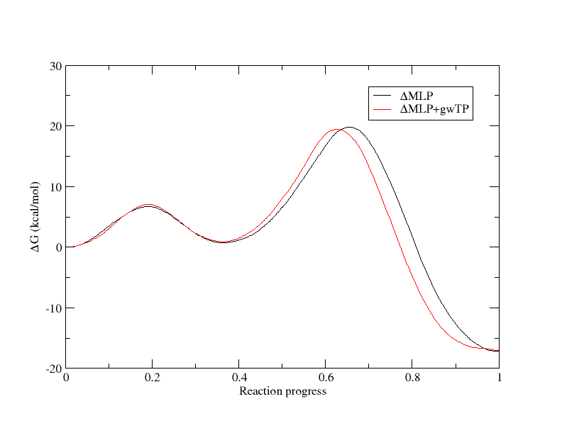
[user@cluster] xmgrace -block path.5.opt.dat.wavg.5.dat -bxy 2:5 -block path.9.opt.dat.wavg.9.dat -bxy 2:5 In the below plot the profiles have been aligned at y=0 for direct comparison.

The profiles are quite similar, with the machine learning potential yielding a rate determining barrier of 19.78 kcal/mol, and gwTP yielding a barrier of 19.43 kcal/mol, but there is still some discrepancy. How well did the machine learning potential do to correct DFTB3 to replicate PBE0? When gwTP is performed, the ndfes program computes an important metric called the reweighting entropy (RE). This is a number between 0 and 1 that effectively quantifies the phase space overlap between the reference and target potential in the bin containing a given point.
  1   0.00000000000000e+00  -8.63471000000000e-01  -1.70990200000000e+00   1.790454e+01        0.095    0.829    145
  2   3.22580645161290e-02  -7.23643099393740e-01  -1.64755575292408e+00   1.826003e+01        0.092    0.847    300
  3   6.45161290322581e-02  -5.74876111556158e-01  -1.61191468070361e+00   1.921170e+01        0.097    0.648    321
  4   9.67741935483871e-02  -4.21798346974683e-01  -1.60630825824268e+00   2.088689e+01        0.122    0.842    556
  5   1.29032258064516e-01  -2.68708585473426e-01  -1.61432636055140e+00   2.278483e+01        0.099    0.791    383
  6   1.61290322580645e-01  -1.15924404582858e-01  -1.62700192661683e+00   2.434311e+01        0.071    0.846    306
  7   1.93548387096774e-01   3.67214780017976e-02  -1.64125858889227e+00   2.496843e+01        0.083    0.842    322
  8   2.25806451612903e-01   1.89328263466230e-01  -1.65592773471958e+00   2.414705e+01        0.077    0.838    256
  9   2.58064516129032e-01   3.42146139061666e-01  -1.66816784509145e+00   2.256895e+01        0.071    0.801    389
 10   2.90322580645161e-01   4.95381667938472e-01  -1.67114524485306e+00   2.095009e+01        0.087    0.699    210
 11   3.22580645161290e-01   6.45897165007477e-01  -1.64514630902587e+00   1.966024e+01        0.077    0.740    200
 12   3.54838709677419e-01   7.70670034331531e-01  -1.55989348185740e+00   1.892839e+01        0.072    0.825    459
 13   3.87096774193548e-01   8.37355743310727e-01  -1.42362410262515e+00   1.887799e+01        0.070    0.825    414
 14   4.19354838709677e-01   8.58090289608902e-01  -1.27193527731017e+00   1.969304e+01        0.089    0.699    377
 15   4.51612903225806e-01   8.61387996286766e-01  -1.11866117045908e+00   2.119472e+01        0.068    0.756    553
 16   4.83870967741935e-01   8.63466229459934e-01  -9.65365197452351e-01   2.335955e+01        0.072    0.726    253
 17   5.16129032258065e-01   8.66744262006695e-01  -8.12090178204530e-01   2.628068e+01        0.088    0.621    408
 18   5.48387096774194e-01   8.68883904826271e-01  -6.58798066066249e-01   2.956726e+01        0.103    0.592    431
 19   5.80645161290323e-01   8.68203679481171e-01  -5.05489469117158e-01   3.345300e+01        0.125    0.511    344
 20   6.12903225806452e-01   8.67317707049999e-01  -3.52181808827297e-01   3.648824e+01        0.070    0.828    385
 21   6.45161290322581e-01   8.66416734393529e-01  -1.98874235948492e-01   3.731200e+01        0.079    0.824    343
 22   6.77419354838710e-01   8.65659808921910e-01  -4.55658939520789e-02   3.582405e+01        0.084    0.737    388
 23   7.09677419354839e-01   8.65081886340590e-01   1.07743222319750e-01   3.197438e+01        0.093    0.734    533
 24   7.41935483870968e-01   8.64941995741777e-01   2.61053313440053e-01   2.643022e+01        0.137    0.500    280
 25   7.74193548387097e-01   8.65433249788374e-01   4.14362165206138e-01   2.056916e+01        0.081    0.711    374
 26   8.06451612903226e-01   8.67806367225160e-01   5.67653537891631e-01   1.471830e+01        0.071    0.643    559
 27   8.38709677419355e-01   8.70841279609953e-01   7.20933592533481e-01   9.755915e+00        0.077    0.754    597
 28   8.70967741935484e-01   8.70576649560447e-01   8.74235322866040e-01   5.873653e+00        0.105    0.703    744
 29   9.03225806451613e-01   8.66137718710170e-01   1.02748030920223e+00   3.391863e+00        0.101    0.677    268
 30   9.35483870967742e-01   8.63563899338629e-01   1.18076636418764e+00   1.937446e+00        0.066    0.828    586
 31   9.67741935483871e-01   8.69235713509602e-01   1.33394269778577e+00   1.305873e+00        0.068    0.702    248
 32   1.00000000000000e+00   8.81511000000000e-01   1.48675000000000e+00   1.025874e+00        0.060    0.731    239
The columns of the file correspond to the index of the point, the progress value, RC1, RC2, the free energy in kcal/mol, the standard error from bootstrap analysis, the RE, and the number of samples in the bin containing the point. Let's focus on the RE's.
[user@cluster] awk '{print $7}' path.9.RE.dat.wavg.9.dat
0.829
0.847
0.648
0.842
0.791
0.846
0.842
0.838
0.801
0.699
0.740
0.825
0.825
0.699
0.756
0.726
0.621
0.592
0.511
0.828
0.824
0.737
0.734
0.500
0.711
0.643
0.754
0.703
0.677
0.828
0.702
0.731[user@cluster] awk '{total += $7} END {print total/NR}' path.9.RE.dat.wavg.9.dat
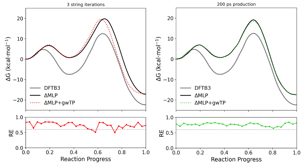
0.739062The average RE is about 0.74, which indicates generally good phase space overlap. A good rule of thumb is that the RE should generally be above 0.6 to be considered a reliable estimate. If many points yield RE below 0.6 you will likely see a noisy PMF, indicating that either the machine learning model is poor, or you need additional sampling. The lower the RE, the more samples will be needed to make a reliable estimate. In this case, there are 3 points that yield RE less than 0.6, with the lowest being 0.5. These points occur on either side of the rate determining transition state, which are areas where the black and red profiles did not align as well. It makes sense that phase space overlap in these regions is imperfect and that gwTP makes the most significant correction here, thus reducing the RE.
In practice, one could run the simulations longer until the RE is no longer increasing. In the below figure, the PMF and resulting RE's from this tutorial (left) are compared the the results after performing gwTP with an additional 200 ps of production sampling on the final path (right).

When exhaustive sampling is performed, all of the REs are above 0.6, and the machine learning and gwTP corrected curves match up nicely. It is difficult to validate a ΔMLP directly by comparing it to ab initio sampling because long-timescale sampling is intractable at the ab initio level. One may compare short time-scale sampling, but such PMFs will typically not represent equilibrium ensembles and may not be an accurate comparison. Therefore, gwTP is a valuable method of validation that avoids any costly ab initio dynamics while collecting equilibrium statistics. The ndfes-CheckEquil.py script in FE-ToolKit is a valuable tool to assess whether an umbrella sampling simulation has reached equilibrium.
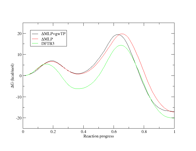
In a previous session, you analyzed string simulations generated at the semi-empirical DFTB3 level. Here we will compare the difference in the PMF at the semi-empirical and your gwTP approximated ab initio level. You have been provided a file called DFTB3.dat in your gwTP directory. DFTB3.dat is the path file that we previously obtained when analyzing the DFTB3 strings that converged to the minimum free energy path. We will compare the machine learning and gwTP corrected PMFs with that of DFTB3 and PBE0.
[user@cluster] xmgrace -block path.9.opt.dat.wavg.9.dat -bxy 2:5 -block path.5.opt.dat.wavg.5.dat -bxy 2:5 -block DFTB3.dat -bxy 2:5 
The PMFs have been aligned at y=0 for direct comparison. First let's focus on the ΔMLP+gwTP (black) and ΔMLP (red) curves. In general, both PMFs produce the same free energy trend with some discrepancies, and as we saw in the above figure, running the simulations for longer would have aided our estimate. Now let's focus on the DFTB3 (green) compared to the high level PMFs. Not only are the rate determining free energy barriers different, but the mechanistic interpretation is different when the higher level of theory is used. At the DFTB3 level (green) there is a stable intermediate state in which the proton transfer has occurred. This would suggest a proton would reside on the ligand a majority of the time. At the approximate PBE0 level, the intermediate is slightly higher in energy than the reactant state, suggesting the proton would likely be in rapid equilibrium between the cytosine residue and the ligand. This has implications for how one would interpret experimental observables such as pH dependence and highlights the importance of balancing the speed of the simulations with the accuracy of the Hamiltonian.