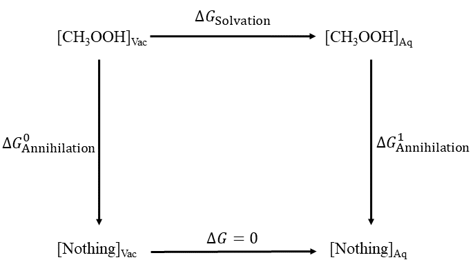
This tutorial will demonstrate how to calculate the absolute solvation free energy of a small molecule using the DDBoost package [ Ganguly 2022]. Solvation free energies are fundamental thermodynamic quantities that are related to a number of physical properties, such as pKₐ, that can have broad implications on rational drug design. A thermodynamic cycle (Fig. 1) is used to determine the absloute solvation free energy.

This involves the annihilation of a molecule to an ideal gas in each of the gas and condensed phases, that is, transition the molecule from its real state (λ=0) to its dummy state (λ=1), where the molecule is decoupled from its enviornment and the intramolecular interactions are scaled. Because the total free energy of a closed thermodynamic cycle must be zero, the solvation energy is thus determined by:
\[ \Delta\mathit{G}_{\mathrm{Solvation}} = \Delta\mathit{G}_{\mathrm{Annihilation}}^{1} - \Delta\mathit{G}_{\mathrm{Annihilation}}^{0} \]
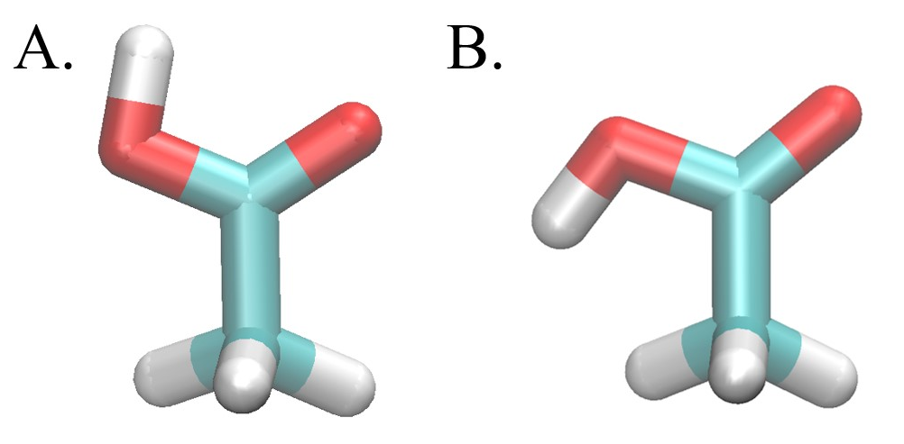
Acetic acid will be the small molecule used in this tutorial. Notably, acetic acid establishes an intramolecular hydrogen bonding interaction in the gas phase, thus orienting the carboxylic acid group in a syn conformation (Fig. 2A), that is not present in the aqueous phase, where the carboxylic acid is arranged in an anti conformation (Fig. 2B).
Energy barriers between the syn and anti conformation as a function of the (O=C-O-H) torsion angle are ~11.0 and ~6.5 kcal/mol in the gas and solution phases respectively [ Lim 2019 ]. These high conformational barriers may persist even in the dummy state (λ=1) depending on the way the dummy state is defined. The SC transforming separable coordinate/softcore) region for an absolute solvation free energy calculation will involve the entire small molecule meaning that the dummy states in both the gas and solution phase are identical. If the internal interactions of the acetic acid molecule are not scaled (SC1), the conformational transition in the dummy state will maintain the energy barrier of the the transition of the real state in the gas phase. Alternatively, if internal electrostatics are scaled to zero (SC2), the dummy state conformational transition will produce an energy barrier more consistent with that of the real state in the solution phase. In order to find the correct absolute solvation free energy, we must account for the transition from the syn to the anti conformation and sample the relevant phase space across the transition pathway. We will do this using the alchemical enhanced sampling (ACES) method. The ACES method involves the use of SC25, where the internal LJ interactions, excluding the 1-4 LJ, bond length, and bond angle energy terms are kept in the dummy state. This treatment eliminates the energy barrier for the dihedral torsion angle around single bonds; thus enabling an enhanced sampled state. The ACES method then uses Hamiltonian replica exchange molecular dynamics (HREMD) to enable further conformational sampling in the real state.
We will look to replicate the simulations described in the paper: ACES: Optimized Alchemically Enhanced Sampling for the absolute hydration free energy of acetic acid [ Lee 2023] with a few modifications. This will involve using the general amber force force field, an OPC water box extending 12 Å from the ligand, and 24, linearly spaced alchemical states ranging from the real state a λ = 0.0 to the dummy state at λ = 1.0. In place of the four, 6 ns long individual trials, this tutorial involves running a single, 1.2 ns simulation that we refer to a "burn-in" simulation. Burn-in simulation are used to optimize the λ-schedule, allowing user to reduce the number of lambda windows, therby increasing computational efficiency.
To begin, let us prepare some directories. First, make a directory called ASFETutorial. Enter this directory and make a directory called "initial". Inside of this directory, make a new directory called AceticAcid. We will copy files prepared during the "Preparing a Small Molecule from PDB to Simulation" tutorial. Copy acetic_acid.mol2, acetic_acid.frcmod, and acetic_acid.lib to this new directory. Rename each file to have the name acetic_acid_0 followed by the file extension.
Now we can use the FE-Workflow tool in the DDBoost package to prepare our system for the necessary simulations. Exit the "initial/AceticAcid" directory. In the ASFETutorial/ make a new direcory called "asfe". Enter this direcotry directory and place the file "input", which can be downloaded here. In the event that you are unable to download this file, you should be able to find a generic input file in your FE-Workflow directory.
Open the input file and ensure that the following key options are set:
path_to_input=../initial
system=AceticAcid
ticalc=asfe
translist=(acetic_acid)
pff=ff19SB
lff=gaff2
wm=opc
ionconc=0.15
twostate=false
ntrials = 1
nstlimti=5
numexchgti=60000
hmr=true
gti_add_sc=25
Now run the following command:
setup_fe
The workflow will now spend some time preparing the system and generating all of the input files needed for analysis in the following steps:
Go to the /path/to/ASFETutorial/asfe/AceticAcid/unified/run/acetic_acid/aq/ directory. A file called "run_alltrials.slurm" should have been created. This file is a job submission script for a computing cluster using the SLURM scheduler. It will need to be modified if you intend to run your program using another scheduler, such as MOAB, or run directly as a shell script. If one wishes to run the script on SDSC's Expase, the "#SBATCH -A <<project*>>" line must be added. Once the necessary modifications have been made, you can run the program. Users at the SDSC free energy workshop can skip ahead to the "Perform Analysis using edgembar" section and copy the data produced by the following steps. For example, if your computing cluster uses the SLURM scheduler:
sbatch run_alltrials.slurm
This will launch a series of simulations :
The workflow will now spend some time preparing the system and generating all of the input files needed for analysis in the following steps:
Go to the path/to/ASFETutorial/ directory and open the input file using a text editor of your choice. Set the following options:
stage=analysis
path_to_data=/path/to/ASFETutorial/asfe/AceticAcid/unified/run
if you have experimental data for your small molecule(s), you can enter the data in a file "Expt.dat" in the format:
name_in_translist expt_value
and set the option:
exptdatafile=Expt.dat
If there is no experimental data available, set the option:
exptdatafile=skip
For acetic acid, the Expt.dat file should look like:
acetic_acid -6.69
Now, perform the analysis using:
setup_fe
The workflow has been setup to automatically perform analysis using the edgembar tools; however, interested readers may wish to further control analysis by directly calling edgembar tools instead of using the workflow for analysis. The first step of edgembar would be to extract the relevant data from the mdout files using edgembar-amber2dats.py. Currently, the workflow will use the command:
edgembar-amber2dats.py -r ${path_out}/../remt1.log --odir=${path_out} $(ls ${path_data}/*ti.mdout)
Where ${path_data} is the path to the mdout files and ${path_out} is the location where data files should be written. Use this command for each trial in both the solution and gas phase. Other options that could be added to the edgembar-amber2dats.py command would be:
The edgembar-amber2dats.py command will extract data from the output file in ${path_data}. The files extracted to ${path_out} will fall into two general formats. dvdl_LAM.dat, where LAM is a λ value for which there is an output, contains the partial derivative of the potential energy with respect to λ. This data is used to determine the ASFE by thermodynamic integration (TI). Files will also be produced to follow the efep_LAM1_LAM2.dat format. These files will contain the energy for the conformations produced at λ=LAM1 using a λ=LAM2 value for the Hamiltonian. These files will be used to determine the ASFE using MBAR.
The extracted data files are available for SDSC users at /expanse/projects/qstore/amber_ws/tutorials/AFE_acetic_acid/results. Note that for our own convience, we have renamed results/data/acetic_acid to results/data/acetic_acid_vac~acetic_acid_aq. Additionally, we are providing data for 4 independent trials of 6 ns so that we can perform analysis on production runs. Next, open a text editor and prepare a file called DiscoverEdges.py:
#!/usr/bin/env python3import edgembarimport osfrom pathlib import Pathodir = Path("analysis")s = r"data/{edge}/{env}/{trial}/efep_{traj}_{ene}.dat"exclusions=Noneedges = edgembar.DiscoverEdges(s, exclude_trials=exclusions, target="aq", reference="vac")if not odir.is_dir(): os.makedirs(odir)for edge in edges: for trial in edge.GetAllTrials(): trial.reverse() fname = odir / (edge.name + ".xml") edge.WriteXml(fname)
DiscoverEdges.py will be used to write information about the data structure used to store our data. Run this code using:
python DiscoverEdges.py
This step is used to create a set of xml files that describe the directory format used to store the data and the λ values where MD was preformed. Then, use the following commands to calculate the free energy and prepare an html report:
OMP_NUM_THREADS=4 edgembar_omp --halves --fwdrev "analysis/acetic_acid_vac~acetic_acid_aq.xml"edgembar-WriteGraphHtml.py -o analysis/Graph.html $(ls analysis/*~*.py)cd analysispython acetic_acid_vac~acetic_acid_aq.py
During these steps, edgembar uses the previously mentioned dvdl_LAM.dat and efep_LAM1_LAM2.dat files to calculate the ASFE. The data is stored in a set of py files, that are then converted into html files for analysis. More details on using edgembar can be found at https://rutgerslbsr.gitlab.io/fe-toolkit/edgembar/index.html.
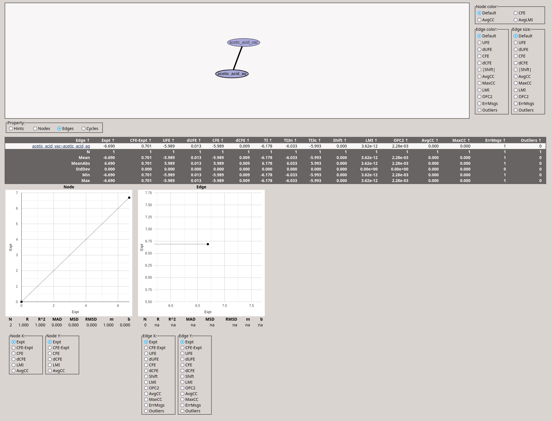
The data will be written to files in the /path/to/ASFETutorial/asfe/results/analysis/ directory. Here, there should be two .html files: Graph.html and acetic_acid_vac~acetic_acid_aq.html.
You can open these files in a web browser. They should look like this:
Now that we've completed our burn-in simulations, we will aim to optimize our λ schedule to maximize efficieny and replica exchange frequency, thereby maximizing the degree of enhanced sampling. [ Zhang 2024].
To do this, we will use the fekutils-tischedule.py tool in fe-toolkit.
fetkutils-tischedule.py --opt 16 --ar --ssc --plot opt_ar_16.png -o opt_ar_16.txt ./data/acetic_acid_vac~acetic_acid_aq/aq/1/
The --opt option allows us to specify the number of λ points we would like to optimize.
The --ar option means that we will use the predicted HREMD acceptance ratio as our optimization criteria.
The --ssc option means that we will optimize two parameters - the order of the SSC function for the first half and second half of the λ schedule as opposed to 16 independent variables for each λ position.
The --plot option is used to generate a graph of the predicted H-REMD acceptance ratios between windows in the optimized λ space (Fig. 4).
The -o option allows us to write the optimized λ schedule to opt_ar_16.txt
Finally, '.' is used to tell fekutils-tischedule.py where the data files are located.
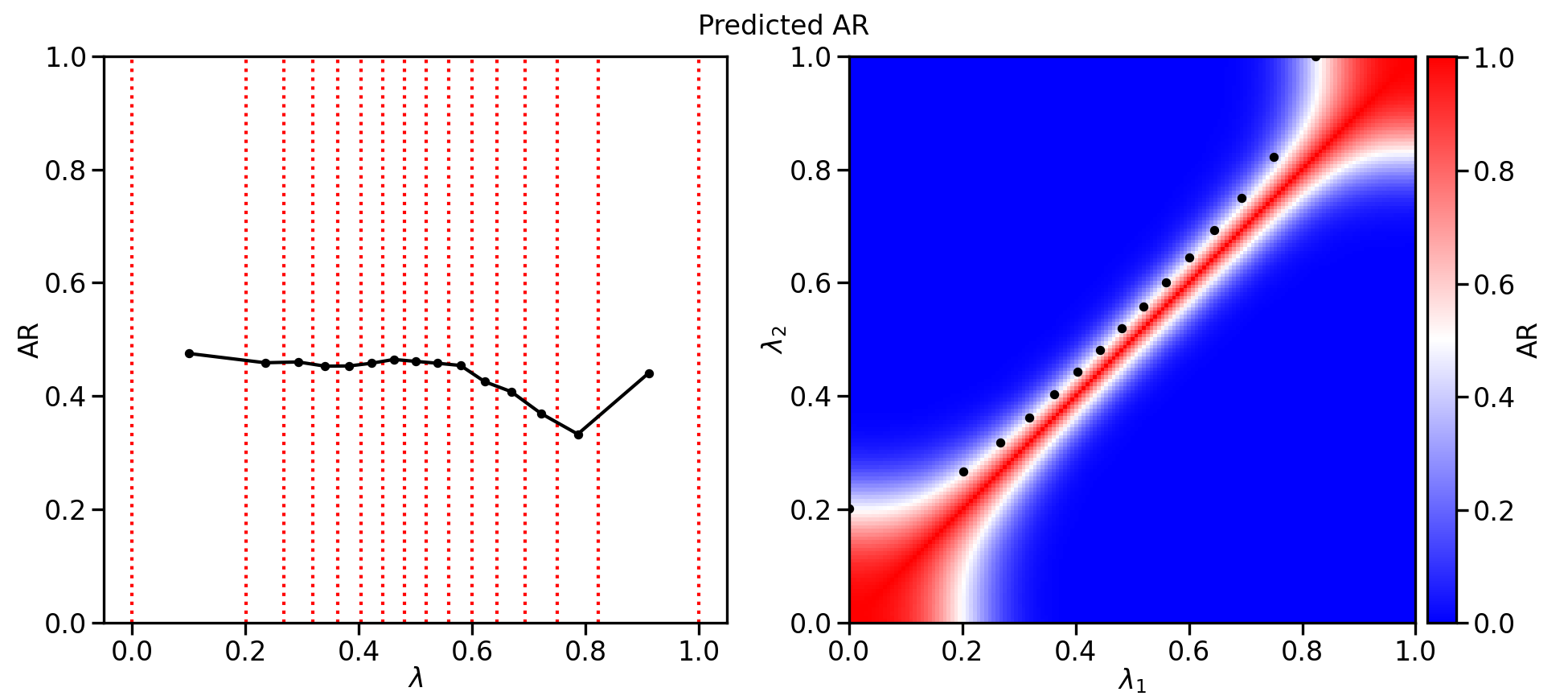
fetkutils-tischedule.py reads data from the efep_LAM1_LAM2.dat files to determine the average probability of a replica exchange between windows at λ=LAM1 and λ=LAM2. These calculated values are interpolated using a radial basis function to be able to predict the probability of a replica exchange between two windows at any λ value. Smooth-step function polynomials for the first (λ=0-0.5) and second (λ=0.5-1.0) halves of the λ are optimized such that a specified number of lambda windows will have predicted H-REMD acceptance ratios as uniformly as possible.
If you use this tutorial, please cite the following papers: